Herbicide applied to Galium aparine
G.aparine.RdSmall plants of Galium aparine, growing in pots in a green house, were sprayed with the technical grade phenmidipham herbicide either alone or in mixture with an ester of oleic acid. The plants were allowed to grow in the green house for 14 days after herbicide treatment. Then the dry matter was measured per pot.
Usage
data(G.aparine)Format
A data frame with 240 observations on the following 3 variables.
dosea numeric vector of dose value (g/ha)
drymattera numeric vector of dry matter weights (mg/pot)
treatmenta numeric vector giving the grouping: 0: control, 1,2: herbicide formulations
Source
Cabanne, F., Gaudry, J. C. and Streibig, J. C. (1999) Influence of alkyl oleates on efficacy of phenmedipham applied as an acetone:water solution on Galium aparine, Weed Research, 39, 57–67.
Examples
library(drc)
## Fitting a model with a common control (so a single upper limit: "1")
G.aparine.m1 <- drm(drymatter ~ dose, treatment, data = G.aparine,
pmodels = data.frame(treatment, treatment, 1, treatment), fct = LL.4())
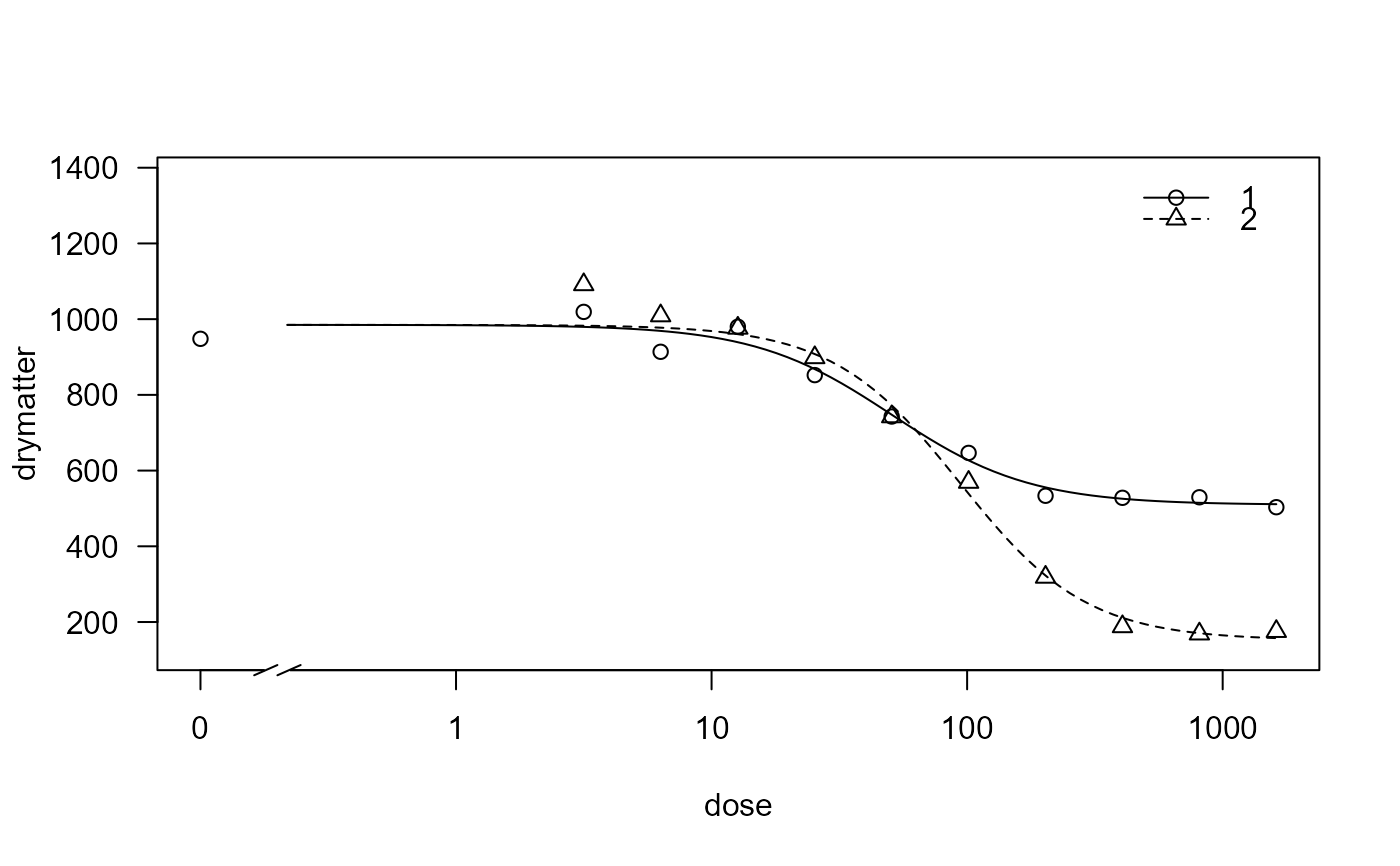
## Visual inspection of fit
plot(G.aparine.m1, broken = TRUE)
 ## Lack of fit test
modelFit(G.aparine.m1)
#> Lack-of-fit test
#>
#> ModelDf RSS Df F value p value
#> ANOVA 219 2601788
#> DRC model 233 2891677 14 1.7429 0.0490
## Summary output
summary(G.aparine.m1)
#>
#> Model fitted: Log-logistic (ED50 as parameter) (4 parms)
#>
#> Parameter estimates:
#>
#> Estimate Std. Error t-value p-value
#> b:1 1.61291 0.33330 4.8392 2.372e-06 ***
#> b:2 1.75100 0.20392 8.5869 1.311e-15 ***
#> c:1 509.50367 23.25885 21.9058 < 2.2e-16 ***
#> c:2 151.91840 26.00899 5.8410 1.734e-08 ***
#> d:(Intercept) 984.88779 12.63335 77.9594 < 2.2e-16 ***
#> e:1 50.80009 7.87851 6.4479 6.467e-10 ***
#> e:2 93.44626 8.11091 11.5211 < 2.2e-16 ***
#> ---
#> Signif. codes: 0 '***' 0.001 '**' 0.01 '*' 0.05 '.' 0.1 ' ' 1
#>
#> Residual standard error:
#>
#> 111.403 (233 degrees of freedom)
## Predicted values with se and confidence intervals
#predict(G.aparine.m1, interval = "confidence")
# long output
## Calculating the relative potency
EDcomp(G.aparine.m1, c(50,50))
#>
#> Estimated ratios of effect doses
#>
#> Estimate Std. Error t-value p-value
#> 1/2:50/50 5.4363e-01 9.3972e-02 -4.8565e+00 2.1923e-06
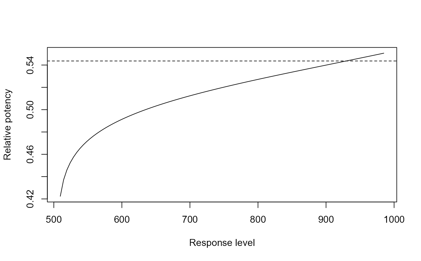
## Showing the relative potency as a
## function of the response level
relpot(G.aparine.m1)
## Lack of fit test
modelFit(G.aparine.m1)
#> Lack-of-fit test
#>
#> ModelDf RSS Df F value p value
#> ANOVA 219 2601788
#> DRC model 233 2891677 14 1.7429 0.0490
## Summary output
summary(G.aparine.m1)
#>
#> Model fitted: Log-logistic (ED50 as parameter) (4 parms)
#>
#> Parameter estimates:
#>
#> Estimate Std. Error t-value p-value
#> b:1 1.61291 0.33330 4.8392 2.372e-06 ***
#> b:2 1.75100 0.20392 8.5869 1.311e-15 ***
#> c:1 509.50367 23.25885 21.9058 < 2.2e-16 ***
#> c:2 151.91840 26.00899 5.8410 1.734e-08 ***
#> d:(Intercept) 984.88779 12.63335 77.9594 < 2.2e-16 ***
#> e:1 50.80009 7.87851 6.4479 6.467e-10 ***
#> e:2 93.44626 8.11091 11.5211 < 2.2e-16 ***
#> ---
#> Signif. codes: 0 '***' 0.001 '**' 0.01 '*' 0.05 '.' 0.1 ' ' 1
#>
#> Residual standard error:
#>
#> 111.403 (233 degrees of freedom)
## Predicted values with se and confidence intervals
#predict(G.aparine.m1, interval = "confidence")
# long output
## Calculating the relative potency
EDcomp(G.aparine.m1, c(50,50))
#>
#> Estimated ratios of effect doses
#>
#> Estimate Std. Error t-value p-value
#> 1/2:50/50 5.4363e-01 9.3972e-02 -4.8565e+00 2.1923e-06
## Showing the relative potency as a
## function of the response level
relpot(G.aparine.m1)
 relpot(G.aparine.m1, interval = "delta")
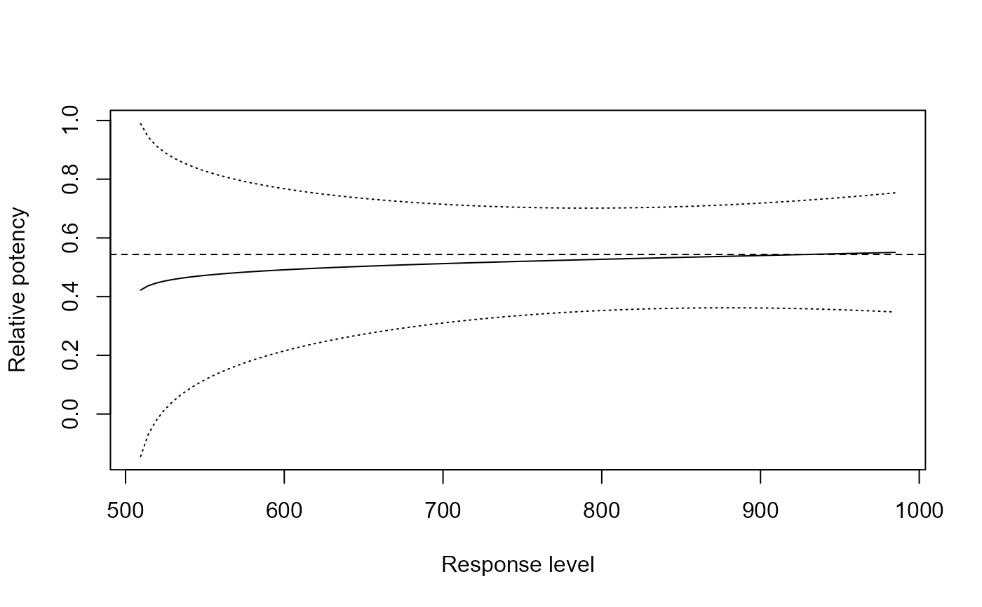 # appears constant!
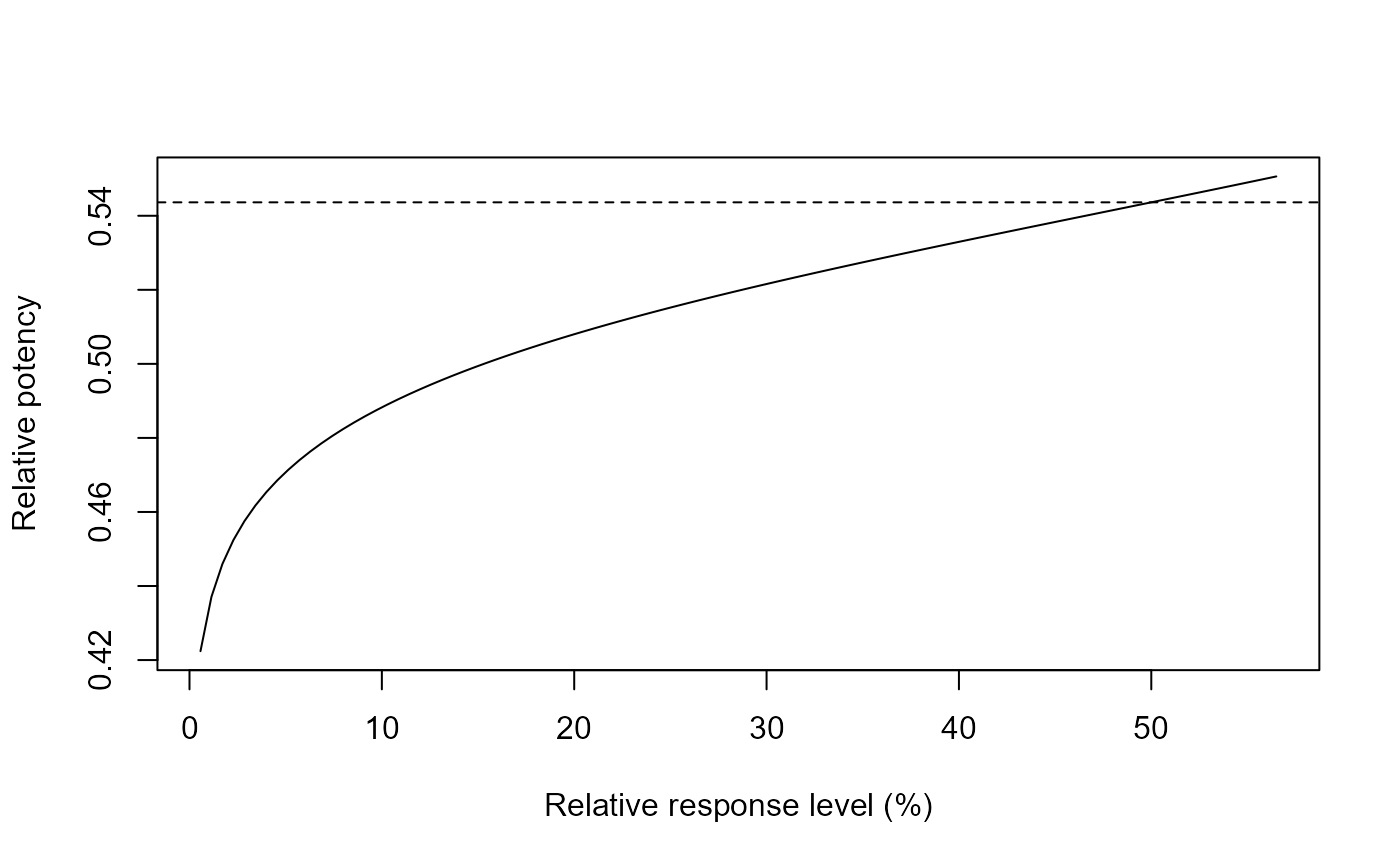
## Response level in percent
relpot(G.aparine.m1, scale = "percent")
# appears constant!
## Response level in percent
relpot(G.aparine.m1, scale = "percent")
 ## Fitting a reduced model (with a common slope parameter)
G.aparine.m2 <- drm(drymatter ~ dose, treatment, data = G.aparine,
pmodels = data.frame(1, treatment, 1, treatment), fct = LL.4())
anova(G.aparine.m2, G.aparine.m1)
#>
#> 1st model
#> fct: LL.4()
#> pmodels: 1, treatment, 1, treatment
#> 2nd model
#> fct: LL.4()
#> pmodels: treatment, treatment, 1, treatment
#>
#> ANOVA table
#>
#> ModelDf RSS Df F value p value
#> 1st model 234 2893283
#> 2nd model 233 2891677 1 0.1294 0.7193
## Showing the relative potency
relpot(G.aparine.m2)
## Fitting a reduced model (with a common slope parameter)
G.aparine.m2 <- drm(drymatter ~ dose, treatment, data = G.aparine,
pmodels = data.frame(1, treatment, 1, treatment), fct = LL.4())
anova(G.aparine.m2, G.aparine.m1)
#>
#> 1st model
#> fct: LL.4()
#> pmodels: 1, treatment, 1, treatment
#> 2nd model
#> fct: LL.4()
#> pmodels: treatment, treatment, 1, treatment
#>
#> ANOVA table
#>
#> ModelDf RSS Df F value p value
#> 1st model 234 2893283
#> 2nd model 233 2891677 1 0.1294 0.7193
## Showing the relative potency
relpot(G.aparine.m2)
 ## Fitting the same model in a different parameterisation
G.aparine.m3 <- drm(drymatter ~ dose, treatment, data = G.aparine,
pmodels = data.frame(treatment, treatment, 1, treatment), fct = LL2.4())
EDcomp(G.aparine.m3, c(50, 50), logBase = exp(1))
#>
#> Estimated ratios of effect doses
#>
#> Estimate Std. Error t-value p-value
#> 1/2:50/50 5.4362e-01 9.3970e-02 -4.8567e+00 2.1904e-06
## Fitting the same model in a different parameterisation
G.aparine.m3 <- drm(drymatter ~ dose, treatment, data = G.aparine,
pmodels = data.frame(treatment, treatment, 1, treatment), fct = LL2.4())
EDcomp(G.aparine.m3, c(50, 50), logBase = exp(1))
#>
#> Estimated ratios of effect doses
#>
#> Estimate Std. Error t-value p-value
#> 1/2:50/50 5.4362e-01 9.3970e-02 -4.8567e+00 2.1904e-06