A Practical Workflow for Dose-Response Analysis

Executive Summary

This vignette provides a comprehensive, step-by-step workflow for conducting proper dose-response analysis using the drc package. We demonstrate the complete analysis process from initial model fitting through model selection, validation, and interpretation. By following this workflow, even inexperienced users can perform rigorous dose-response modeling while avoiding common pitfalls.

Introduction

Dose-response analysis is fundamental in toxicology, ecotoxicology, pharmacology, and related fields. The relationship between dose (or concentration) and biological response often follows non-linear patterns that require specialized statistical models. The drc package provides a comprehensive framework for fitting, comparing, and interpreting dose-response models.

What You Will Learn

This vignette demonstrates a complete workflow including:

Initial exploratory model fitting
Visual assessment of model adequacy
Statistical evaluation of model fit
Systematic model comparison and selection
Model-averaged estimation for robust inference
Understanding the impact of parameter constraints
Choosing appropriate models for different data types

The Example Dataset

We will use the ryegrass dataset, which contains measurements of root length in perennial ryegrass (Lolium perenne L.) exposed to different concentrations of ferulic acid, a phenolic compound that inhibits plant growth.

# Load the ryegrass dataset
data(ryegrass)

# Examine the data structure
head(ryegrass, 10)
#>       rootl conc
#> 1  7.580000 0.00
#> 2  8.000000 0.00
#> 3  8.328571 0.00
#> 4  7.250000 0.00
#> 5  7.375000 0.00
#> 6  7.962500 0.00
#> 7  8.355556 0.94
#> 8  6.914286 0.94
#> 9  7.750000 0.94
#> 10 6.871429 1.88

# Summary statistics
summary(ryegrass)
#>      rootl             conc       
#>  Min.   :0.2200   Min.   : 0.000  
#>  1st Qu.:0.8491   1st Qu.: 0.705  
#>  Median :5.0778   Median : 2.815  
#>  Mean   :4.3272   Mean   : 7.384  
#>  3rd Qu.:7.4262   3rd Qu.: 9.375  
#>  Max.   :8.3556   Max.   :30.000

# Simple exploratory plot
plot(rootl ~ conc, data = ryegrass,
     xlab = "Ferulic acid concentration (mM)",
     ylab = "Root length (cm)",
     main = "Ryegrass Root Growth vs. Ferulic Acid Concentration",
     pch = 16, cex = 1.2)

The dataset contains 24 observations with: - conc: Ferulic acid concentration in millimolar (mM) - rootl: Root length in centimeters (cm)

We observe a clear dose-response relationship: as the concentration increases, root length decreases, indicating an inhibitory effect of ferulic acid on ryegrass root growth.

Step 1: Initial Model Fitting

Choosing a Starting Model

For a typical monotonic dose-response curve, the four-parameter log-logistic model (LL.4) is an excellent starting point. It is flexible, well-characterized, and commonly used in toxicology.

The LL.4 model has the form:

$f(x) = c + \frac{d-c}{1 + \exp(b(\log(x) - \log(e)))}$

where: - b: Slope parameter (steepness of the curve) - c: Lower asymptote (response at infinite dose) - d: Upper asymptote (response at zero dose, control response) - e: ED50 or EC50 (dose producing 50% of the maximal effect)

Fitting the Initial Model

# Fit a four-parameter log-logistic model
ryegrass.LL4 <- drm(rootl ~ conc, data = ryegrass, fct = LL.4())

# Display model summary
summary(ryegrass.LL4)
#> 
#> Model fitted: Log-logistic (ED50 as parameter) (4 parms)
#> 
#> Parameter estimates:
#> 
#>               Estimate Std. Error t-value   p-value    
#> b:(Intercept)  2.98222    0.46506  6.4125 2.960e-06 ***
#> c:(Intercept)  0.48141    0.21219  2.2688   0.03451 *  
#> d:(Intercept)  7.79296    0.18857 41.3272 < 2.2e-16 ***
#> e:(Intercept)  3.05795    0.18573 16.4644 4.268e-13 ***
#> ---
#> Signif. codes:  0 '***' 0.001 '**' 0.01 '*' 0.05 '.' 0.1 ' ' 1
#> 
#> Residual standard error:
#> 
#>  0.5196256 (20 degrees of freedom)

The summary provides: - Parameter estimates and their standard errors - Residual standard error - Model convergence information

Interpretation of Parameters: - The d parameter (upper limit) represents the control root length (at zero concentration) - The c parameter (lower limit) represents the minimum root length at high concentrations - The e parameter (ED50) is the concentration causing 50% reduction from control - The b parameter controls the steepness of the dose-response curve

Step 2: Visual Assessment of Model Fit

Visual diagnostics are crucial for assessing whether the fitted model adequately describes the data. We use two primary tools: the standard dose-response plot and quantile-quantile (Q-Q) plots.

Standard Dose-Response Plot

# Plot the fitted model with data points
plot(ryegrass.LL4, type = "all",
     main = "LL.4 Model Fit to Ryegrass Data",
     xlab = "Ferulic acid concentration (mM)",
     ylab = "Root length (cm)",
     lwd = 2, cex = 1.2)

The plot shows: - Observed data points - Fitted dose-response curve - Overall pattern of fit

What to Look For: - Do the fitted values follow the general trend of the data? - Are there systematic deviations (e.g., all points above or below the curve in certain regions)? - Are there outliers that might influence the fit?

Quantile-Quantile (Q-Q) Plot

Q-Q plots assess whether the model residuals follow a normal distribution, which is an assumption of the fitting procedure.

# Create Q-Q plot for residual diagnostics
qqnorm(residuals(ryegrass.LL4),
       main = "Normal Q-Q Plot of Residuals (LL.4)",
       pch = 16, cex = 1.2)
qqline(residuals(ryegrass.LL4), col = "red", lwd = 2)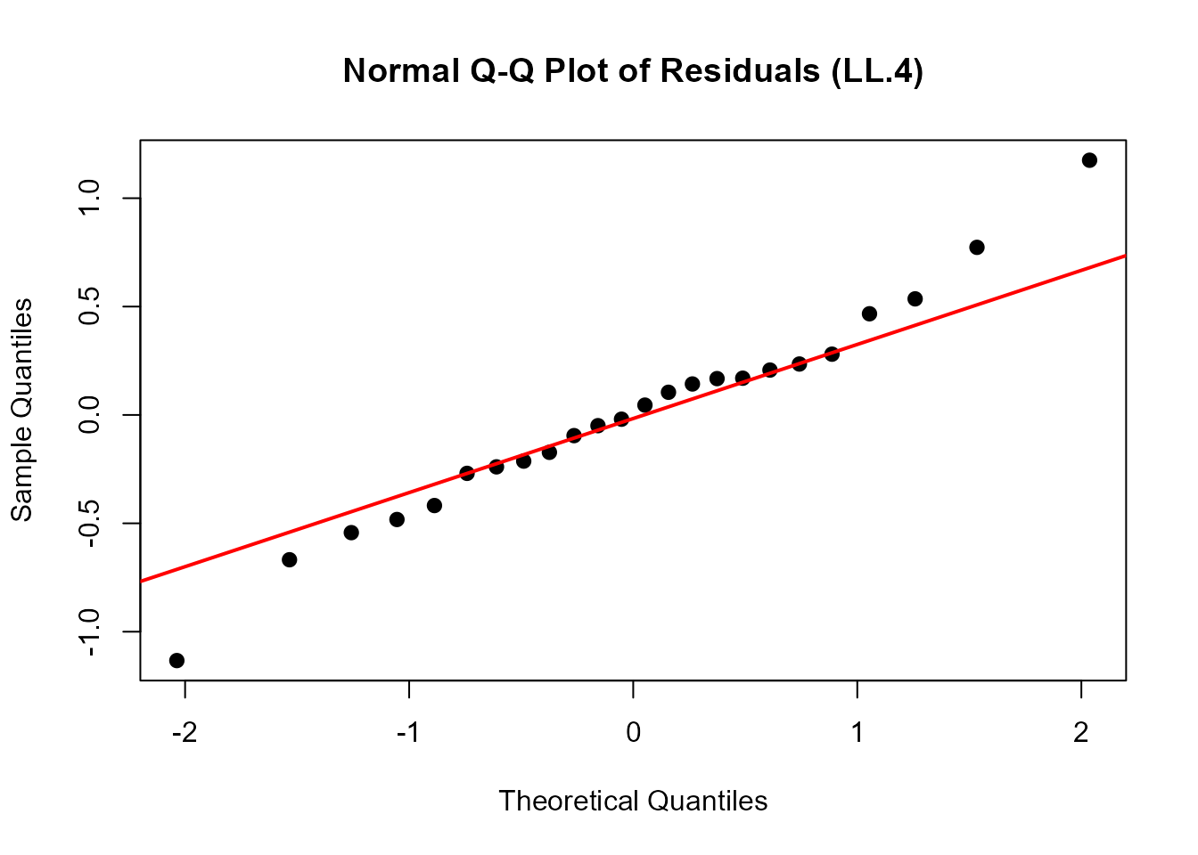

Interpretation: - Points should fall approximately along the diagonal line - Systematic deviations suggest non-normality of residuals - Deviations at the extremes are common and often acceptable - Severe deviations may indicate model inadequacy or outliers

Residual Plot

An additional useful diagnostic is plotting residuals against fitted values:

# Residuals vs. Fitted values
plot(fitted(ryegrass.LL4), residuals(ryegrass.LL4),
     xlab = "Fitted values",
     ylab = "Residuals",
     main = "Residual Plot (LL.4)",
     pch = 16, cex = 1.2)
abline(h = 0, col = "red", lwd = 2, lty = 2)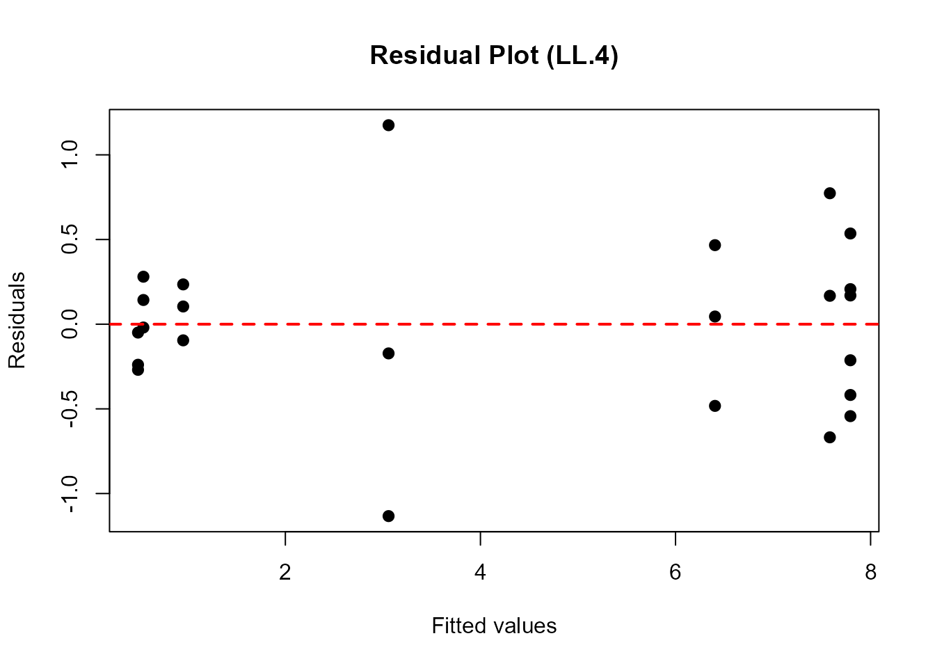

What to Look For: - Random scatter around zero (no systematic pattern) - Constant variance across fitted values (homoscedasticity) - No obvious outliers or influential points

Step 3: Statistical Evaluation of Model Fit

Beyond visual assessment, we use formal statistical tests to evaluate model adequacy and significance.

Test for Dose Effect: noEffect()

The noEffect() function performs a likelihood ratio test comparing the dose-response model to a null model (no dose effect).

# Test whether there is a significant dose effect
noEffect(ryegrass.LL4)
#> Chi-square test              Df         p-value 
#>        91.87776         3.00000         0.00000

Interpretation: - The null hypothesis is “no dose effect” (all responses are equal) - A significant p-value (< 0.05) indicates that the dose-response model fits significantly better than the null model - This confirms that ferulic acid concentration has a significant effect on root length

Goodness-of-Fit Test: modelFit()

The modelFit() function assesses whether the model adequately describes the data using a lack-of-fit test.

# Perform goodness-of-fit test
modelFit(ryegrass.LL4)
#> Lack-of-fit test
#> 
#>           ModelDf    RSS Df F value p value
#> ANOVA          17 5.1799                   
#> DRC model      20 5.4002  3  0.2411  0.8665

Interpretation: - This test compares the fitted model to a saturated model (perfect fit) - A non-significant p-value suggests adequate fit (model is not significantly worse than perfect fit) - A significant p-value indicates lack of fit (model may be inadequate) - Note: This test requires replication at dose levels

Estimating Effective Doses: ED()

Effective dose (ED) or effective concentration (EC) values are key outputs in dose-response analysis. They represent the dose required to produce a specified level of effect.

# Estimate EC10, EC20, and EC50 with 95% confidence intervals
# Using delta method for confidence intervals
ed_values <- ED(ryegrass.LL4, respLev = c(10, 20, 50), interval = "delta")
#> 
#> Estimated effective doses
#> 
#>      Estimate Std. Error   Lower   Upper
#> e:10  1.46371    0.18677 1.07411 1.85330
#> e:20  1.92109    0.17774 1.55032 2.29186
#> e:50  3.05795    0.18573 2.67053 3.44538
ed_values
#>      Estimate Std. Error    Lower    Upper
#> e:10 1.463706  0.1867704 1.074109 1.853302
#> e:20 1.921091  0.1777432 1.550325 2.291857
#> e:50 3.057955  0.1857313 2.670526 3.445384

Understanding ED Values: - EC10: Concentration causing 10% effect (reduction in root length) - EC20: Concentration causing 20% effect - EC50: Concentration causing 50% effect (often used as a summary measure of potency)

Confidence Intervals: - The interval = "delta" argument uses the delta method for CI estimation - Alternative methods include "fls" (fieller), "tfls" (transformed fieller) - Narrower CIs indicate more precise estimates

Alternative Confidence Interval Methods

# Compare different confidence interval methods
cat("Delta method:\n")
#> Delta method:
ED(ryegrass.LL4, respLev = 50, interval = "delta")
#> 
#> Estimated effective doses
#> 
#>      Estimate Std. Error   Lower   Upper
#> e:50  3.05795    0.18573 2.67053 3.44538

cat("\nFieller method:\n")
#> 
#> Fieller method:
ED(ryegrass.LL4, respLev = 50, interval = "fls")
#> 
#> Estimated effective doses
#> 
#>      Estimate  Lower  Upper
#> e:50   21.284 14.448 31.355

The Fieller method is often preferred for ED50 estimation as it accounts for the ratio nature of the parameter.

Step 4: Model Comparison and Selection

A critical step in dose-response analysis is comparing alternative models to select the most appropriate one. Different model families may fit the data better depending on the underlying biological mechanism.

Comparing Multiple Models

We’ll compare the initial LL.4 model with several alternatives:

LN.4: Four-parameter log-normal model
W1.4: Four-parameter Weibull type 1 model
W2.4: Four-parameter Weibull type 2 model
BC.4: Four-parameter Brain-Cousens hormesis model
LL.5: Five-parameter log-logistic model (asymmetric)
EXD.3: Three-parameter exponential decay model

# Use mselect() to compare multiple models
# This fits each model and compares using AIC
model_comparison <- suppressWarnings(
 mselect(
   ryegrass.LL4,
   fctList = list(LN.4(), W1.4(), W2.4(), BC.4(), LL.5(), EXD.3())
   )
 )
model_comparison
#>          logLik       IC Lack of fit   Res var
#> W2.4  -15.91352 41.82703 0.945071314 0.2646283
#> LL.4  -16.15514 42.31029 0.866483043 0.2700107
#> LN.4  -16.29214 42.58429 0.818641010 0.2731110
#> LL.5  -15.87828 43.75656 0.853847582 0.2777393
#> BC.4  -17.05120 44.10241 0.565407254 0.2909448
#> W1.4  -17.46720 44.93439 0.450567622 0.3012075
#> EXD.3 -28.22358 64.44717 0.000886637 0.7030127

Understanding the Output:

The table shows: - logLik: Log-likelihood (higher is better, but penalized for parameters) - IC: Information criterion (AIC by default; lower is better) - Res var: Residual variance (lower is better) - Lack of fit: P-value for lack-of-fit test (non-significant is better)

Models are sorted by IC (AIC), with the best-fitting model at the top.

Selecting the Best Model

# Based on mselect results, fit the best model
# (In this example, we'll use the model with lowest AIC from the comparison)
# For ryegrass data, typically W1.4 or LL.4 performs well

ryegrass.best <- drm(rootl ~ conc, data = ryegrass, fct = W1.4())

# Summary of best model
summary(ryegrass.best)
#> 
#> Model fitted: Weibull (type 1) (4 parms)
#> 
#> Parameter estimates:
#> 
#>               Estimate Std. Error t-value   p-value    
#> b:(Intercept)  2.39341    0.47832  5.0038 6.813e-05 ***
#> c:(Intercept)  0.66045    0.18857  3.5023  0.002243 ** 
#> d:(Intercept)  7.80586    0.20852 37.4348 < 2.2e-16 ***
#> e:(Intercept)  3.60013    0.20311 17.7250 1.068e-13 ***
#> ---
#> Signif. codes:  0 '***' 0.001 '**' 0.01 '*' 0.05 '.' 0.1 ' ' 1
#> 
#> Residual standard error:
#> 
#>  0.5488238 (20 degrees of freedom)

# ED estimates for best model
ed_best <- ED(ryegrass.best, respLev = c(10, 20, 50), interval = "delta")
#> 
#> Estimated effective doses
#> 
#>      Estimate Std. Error   Lower   Upper
#> e:10  1.40598    0.25357 0.87705 1.93491
#> e:20  1.92374    0.23477 1.43403 2.41346
#> e:50  3.08896    0.17331 2.72744 3.45048
ed_best
#>      Estimate Std. Error     Lower    Upper
#> e:10 1.405979  0.2535663 0.8770491 1.934909
#> e:20 1.923744  0.2347672 1.4340283 2.413460
#> e:50 3.088964  0.1733114 2.7274422 3.450485

Visual Comparison of Models

Plotting multiple models together helps visualize differences in fit:

# Plot initial LL.4 model
plot(ryegrass.LL4, type = "all",
     main = "Comparison: LL.4 vs W1.4 Models",
     xlab = "Ferulic acid concentration (mM)",
     ylab = "Root length (cm)",
     lwd = 2, cex = 1.2, col = "blue",
     legend = FALSE)

# Overlay the best model (W1.4)
plot(ryegrass.best, add = TRUE, type = "none", lwd = 2, col = "red", lty = 2)

# Add legend
legend("topright", legend = c("LL.4 (initial)", "W1.4 (best)"),
       col = c("blue", "red"), lwd = 2, lty = c(1, 2), cex = 1.1)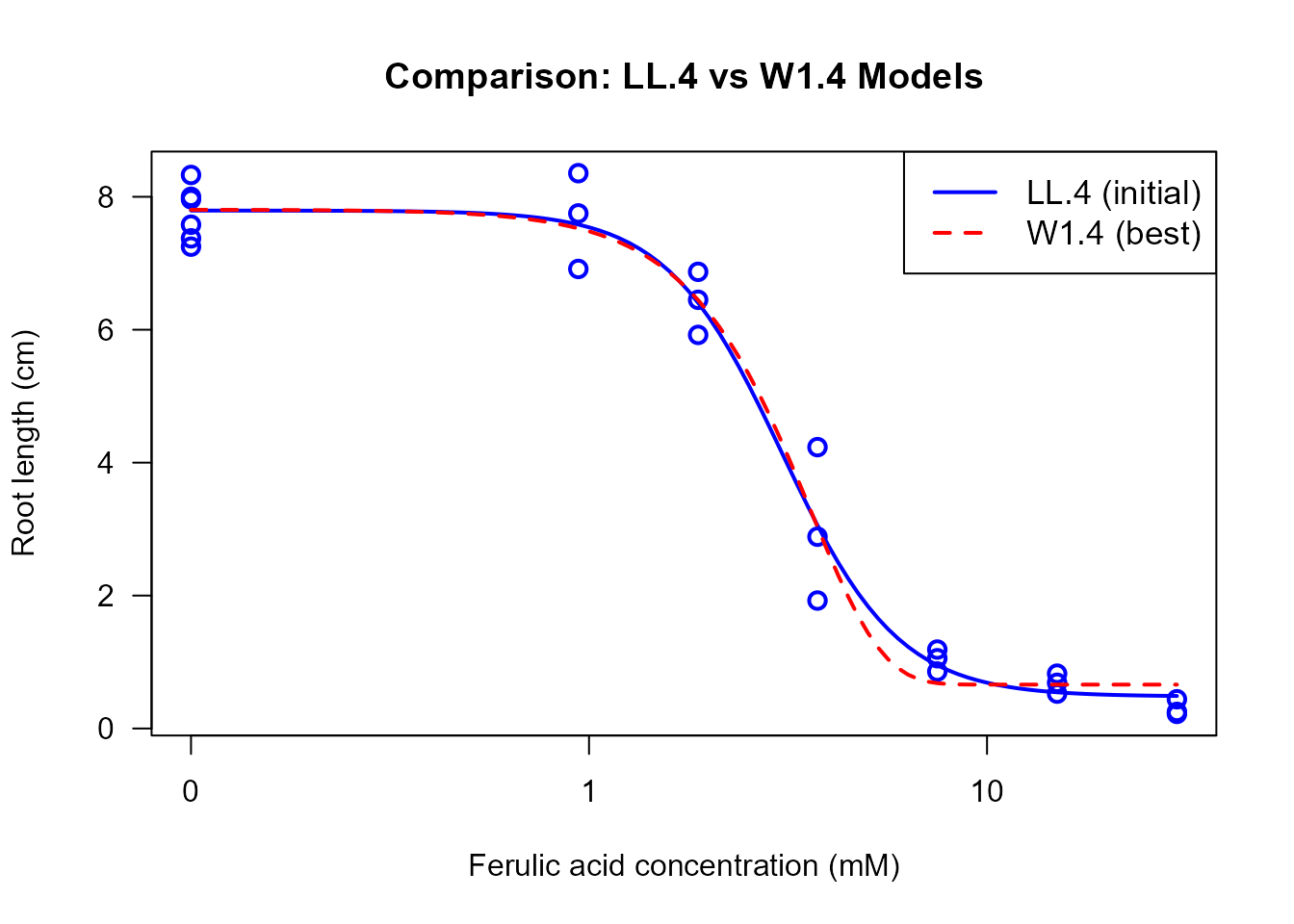

Comparing ED Estimates Between Models

# Compare EC50 estimates between models
cat("EC50 from LL.4 model:\n")
#> EC50 from LL.4 model:
ED(ryegrass.LL4, respLev = 50, interval = "delta")
#> 
#> Estimated effective doses
#> 
#>      Estimate Std. Error   Lower   Upper
#> e:50  3.05795    0.18573 2.67053 3.44538

cat("\nEC50 from W1.4 model:\n")
#> 
#> EC50 from W1.4 model:
ED(ryegrass.best, respLev = 50, interval = "delta")
#> 
#> Estimated effective doses
#> 
#>      Estimate Std. Error   Lower   Upper
#> e:50  3.08896    0.17331 2.72744 3.45048

Important Notes: - Different models may yield different ED estimates - Model selection should be based on both statistical criteria (AIC) and biological plausibility - Small differences in AIC (< 2) suggest models are essentially equivalent

Step 5: Model-Averaged ED Estimation

When multiple models fit similarly well, model averaging provides a robust approach that accounts for model uncertainty. The maED() function computes model-averaged ED estimates using AIC-based weights.

Computing Model-Averaged EDs

# Model-averaged EC50 estimation using top 3 models
# Based on our mselect results, we'll average over several competitive models
ma_results <- maED(ryegrass.LL4,
                   fctList = list(W1.4(), W2.4(), LL.5()),
                   respLev = 50,
                   interval = "buckland")
#>          ED50     Weight
#> LL.4 3.057955 0.33027128
#> W1.4 3.088964 0.08893096
#> W2.4 2.996913 0.42054089
#> LL.5 3.023549 0.16025686

ma_results
#>      Estimate Std. Error    Lower    Upper
#> e:50 3.029528  0.1969989 2.643417 3.415639

Understanding Model Averaging:

Each model receives a weight based on its AIC value
Better-fitting models (lower AIC) receive higher weights
The final estimate is a weighted average across models
Confidence intervals account for both parameter uncertainty and model uncertainty

Comparing Single-Model vs Model-Averaged Estimates

# Compare model-averaged EC50 with single-model estimates
cat("Single model (W1.4) EC50:\n")
#> Single model (W1.4) EC50:
ED(ryegrass.best, respLev = 50, interval = "delta")
#> 
#> Estimated effective doses
#> 
#>      Estimate Std. Error   Lower   Upper
#> e:50  3.08896    0.17331 2.72744 3.45048

cat("\nModel-averaged EC50 (top 3 models):\n")
#> 
#> Model-averaged EC50 (top 3 models):
print(ma_results)
#>      Estimate Std. Error    Lower    Upper
#> e:50 3.029528  0.1969989 2.643417 3.415639

When to Use Model Averaging: - Multiple models have similar AIC values (ΔAIC < 2-4) - You want robust estimates that don’t depend on selecting a single model - Regulatory or risk assessment contexts requiring conservative estimates

When to Use Single Model: - One model is clearly superior (ΔAIC > 10) - Strong biological rationale for a specific model form - Simpler interpretation needed

Step 6: Impact of Fixing Asymptotes

The upper and lower asymptotes (parameters d and c) can be estimated from the data or fixed based on prior knowledge. Understanding when and how to fix these parameters is crucial for proper model fitting.

Understanding Asymptote Parameters

d (upper limit): Response at zero dose (control response)
c (lower limit): Response at infinite dose (maximal effect)

Models with Different Asymptote Constraints

# LL.4: Both asymptotes free (4 parameters)
ryegrass.LL4 <- drm(rootl ~ conc, data = ryegrass, fct = LL.4())

# LL.3: Lower asymptote fixed at 0 (3 parameters)
ryegrass.LL3 <- drm(rootl ~ conc, data = ryegrass, fct = LL.3())

# LL.3u: Upper asymptote fixed at 1 (3 parameters)
# Note: Requires normalized data for this to be meaningful
ryegrass_norm <- ryegrass
ryegrass_norm$rootl_norm <- ryegrass$rootl / max(ryegrass$rootl)
ryegrass.LL3u <- drm(rootl_norm ~ conc, data = ryegrass_norm, fct = LL.3u())

# LL.2: Both asymptotes fixed (2 parameters)
ryegrass.LL2 <- drm(rootl_norm ~ conc, data = ryegrass_norm, fct = LL.2())

# Compare models
cat("LL.4 (both free):\n")
#> LL.4 (both free):
summary(ryegrass.LL4)
#> 
#> Model fitted: Log-logistic (ED50 as parameter) (4 parms)
#> 
#> Parameter estimates:
#> 
#>               Estimate Std. Error t-value   p-value    
#> b:(Intercept)  2.98222    0.46506  6.4125 2.960e-06 ***
#> c:(Intercept)  0.48141    0.21219  2.2688   0.03451 *  
#> d:(Intercept)  7.79296    0.18857 41.3272 < 2.2e-16 ***
#> e:(Intercept)  3.05795    0.18573 16.4644 4.268e-13 ***
#> ---
#> Signif. codes:  0 '***' 0.001 '**' 0.01 '*' 0.05 '.' 0.1 ' ' 1
#> 
#> Residual standard error:
#> 
#>  0.5196256 (20 degrees of freedom)

cat("\nLL.3 (lower = 0):\n")
#> 
#> LL.3 (lower = 0):
summary(ryegrass.LL3)
#> 
#> Model fitted: Log-logistic (ED50 as parameter) with lower limit at 0 (3 parms)
#> 
#> Parameter estimates:
#> 
#>               Estimate Std. Error t-value   p-value    
#> b:(Intercept)  2.47033    0.34168  7.2299 4.011e-07 ***
#> d:(Intercept)  7.85543    0.20438 38.4352 < 2.2e-16 ***
#> e:(Intercept)  3.26336    0.19641 16.6154 1.474e-13 ***
#> ---
#> Signif. codes:  0 '***' 0.001 '**' 0.01 '*' 0.05 '.' 0.1 ' ' 1
#> 
#> Residual standard error:
#> 
#>  0.5615802 (21 degrees of freedom)

cat("\nAIC Comparison:\n")
#> 
#> AIC Comparison:
cat("LL.4 (4 params):", AIC(ryegrass.LL4), "\n")
#> LL.4 (4 params): 42.31029
cat("LL.3 (3 params):", AIC(ryegrass.LL3), "\n")
#> LL.3 (3 params): 45.20827

Visual Comparison of Constrained Models

# Plot models with different constraints
plot(ryegrass.LL4, type = "all",
     main = "Effect of Asymptote Constraints",
     xlab = "Ferulic acid concentration (mM)",
     ylab = "Root length (cm)",
     lwd = 2, col = "black", legend = FALSE, cex = 1.2)

plot(ryegrass.LL3, add = TRUE, type = "none", lwd = 2, col = "blue", lty = 2)

legend("topright",
       legend = c("LL.4 (both free)", "LL.3 (c = 0)"),
       col = c("black", "blue"),
       lwd = 2, lty = c(1, 2),
       cex = 1.1)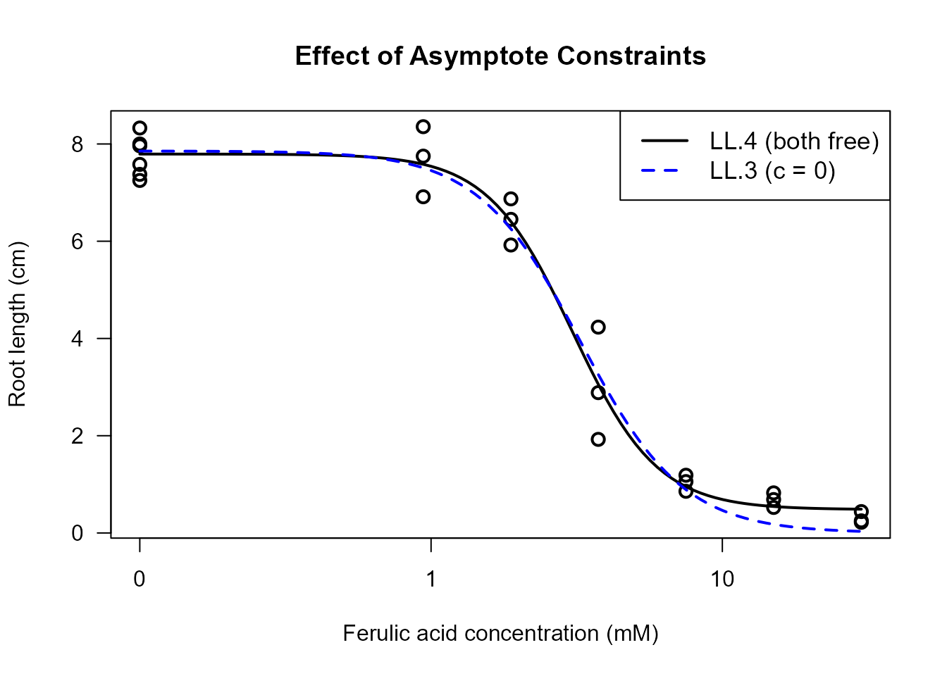

Implications of Fixing Asymptotes

Benefits of Fixing Asymptotes: 1. Reduced parameter count: Simpler model, fewer parameters to estimate 2. Improved stability: Fewer parameters can mean more stable fits 3. Biological relevance: Incorporating prior knowledge (e.g., c = 0 when complete inhibition is impossible) 4. Identifiability: Some datasets may not contain enough information to estimate all parameters

When to Fix Asymptotes: - Fix c = 0 when: - Response cannot go below zero (e.g., growth, survival) - Biological knowledge indicates complete inhibition doesn’t occur - Data doesn’t extend to high enough doses to estimate c

Fix d when:
- Control response is known from independent measurements
- Data is normalized to a known maximum (e.g., 100%)
- You want to focus on relative potency comparisons

When to Keep Asymptotes Free: - Data extends over a wide dose range - Both asymptotes are clearly identifiable in the data - No strong prior knowledge about asymptote values - Model comparison/selection workflow

Effect on ED Estimates

# Compare ED estimates with different constraints
cat("EC50 with LL.4 (both asymptotes free):\n")
#> EC50 with LL.4 (both asymptotes free):
ED(ryegrass.LL4, respLev = 50, interval = "delta")
#> 
#> Estimated effective doses
#> 
#>      Estimate Std. Error   Lower   Upper
#> e:50  3.05795    0.18573 2.67053 3.44538

cat("\nEC50 with LL.3 (lower asymptote = 0):\n")
#> 
#> EC50 with LL.3 (lower asymptote = 0):
ED(ryegrass.LL3, respLev = 50, interval = "delta")
#> 
#> Estimated effective doses
#> 
#>      Estimate Std. Error   Lower   Upper
#> e:50  3.26336    0.19641 2.85491 3.67181

Important Note: The choice of asymptote constraints can substantially affect ED estimates, especially for EC10 and EC20 values which depend more heavily on the asymptote values than EC50.

Step 7: Overview of Available Models

The drc package provides numerous dose-response models suitable for different types of data and biological mechanisms. Understanding which model to use is crucial for proper analysis.

Monotonic (Non-Hormesis) Models

Monotonic models describe dose-response relationships that are either strictly increasing or strictly decreasing. These are appropriate when the response changes consistently in one direction as dose increases.

Log-Logistic Models (LL family)

Characteristics: - Symmetric on log-dose scale - Most commonly used in toxicology - S-shaped curve - Parameters: b (slope), c (lower), d (upper), e (ED50)

Variants: - LL.2(): 2 parameters (c=0, d=1 fixed) - LL.3(): 3 parameters (c=0) - LL.3u(): 3 parameters (d=1) - LL.4(): 4 parameters (most flexible) - LL.5(): 5 parameters (asymmetric, f parameter)

Best for: - General dose-response data - Toxicity studies - EC50/ED50 estimation

Example:

# Standard application of log-logistic model
example.LL <- drm(rootl ~ conc, data = ryegrass, fct = LL.4())
plot(example.LL, main = "Log-Logistic Model (LL.4)")

Weibull Models (W1 and W2 families)

Characteristics: - Asymmetric on log-dose scale - Two types: W1 (increasing asymmetry) and W2 (decreasing asymmetry) - Flexible shape - Same parameter structure as log-logistic

Variants: - W1.2(), W1.3(), W1.4(): Weibull type 1 - W2.2(), W2.3(), W2.4(): Weibull type 2

Best for: - Data with asymmetric dose-response curves - Time-to-event data - Germination/mortality studies

Example:

# Weibull models often fit plant growth data well
example.W1 <- drm(rootl ~ conc, data = ryegrass, fct = W1.4())
example.W2 <- drm(rootl ~ conc, data = ryegrass, fct = W2.4())

# Compare
plot(example.W1, type = "all", main = "Weibull Type 1 vs Type 2",
     lwd = 2, col = "blue", legend = FALSE)
plot(example.W2, add = TRUE, type = "none", lwd = 2, col = "red", lty = 2)
legend("topright", legend = c("W1.4", "W2.4"),
       col = c("blue", "red"), lwd = 2, lty = c(1, 2))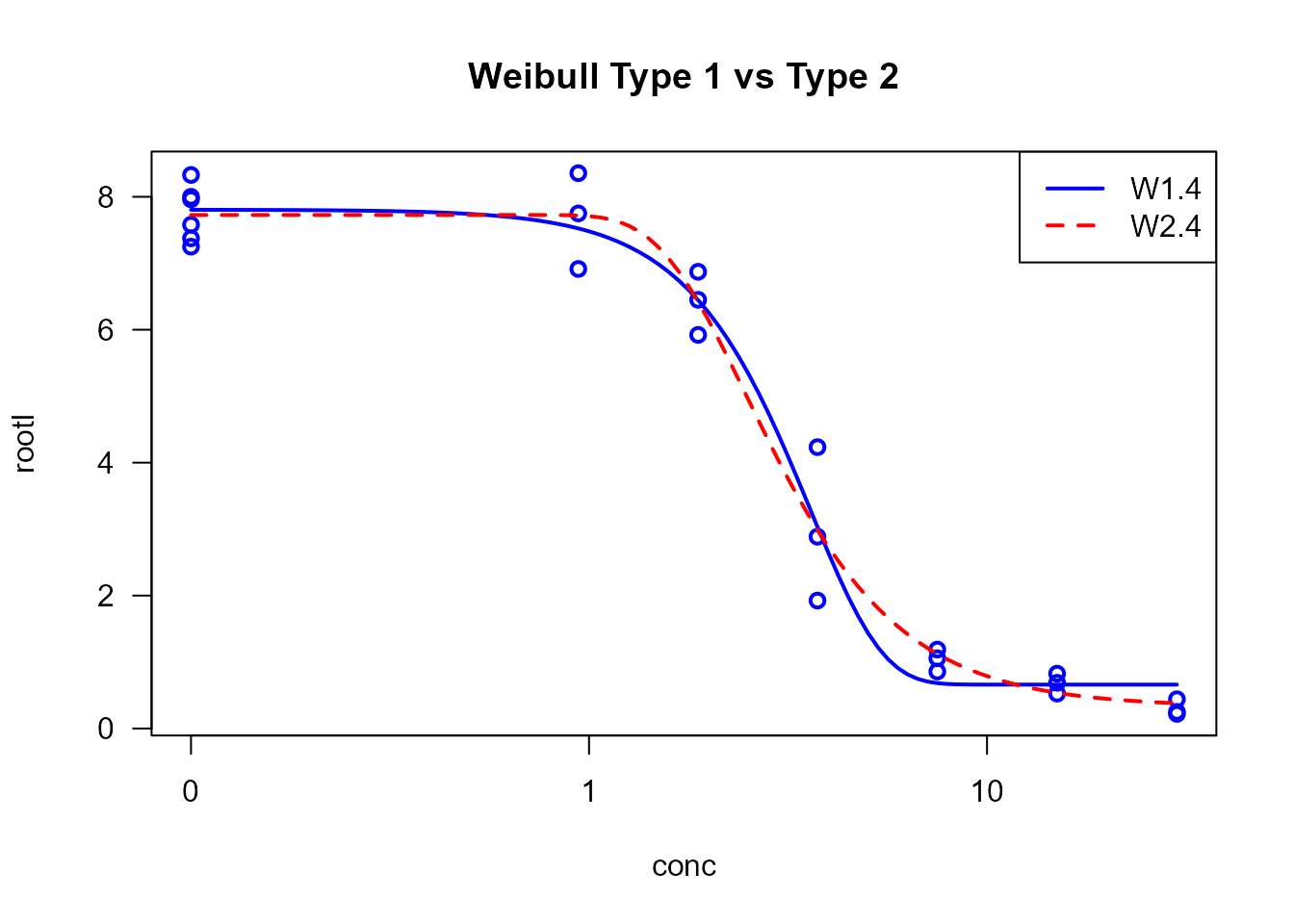

Log-Normal Models (LN family)

Characteristics: - Based on log-normal distribution - Symmetric on log-dose scale - Similar to log-logistic but different tail behavior

Variants: - LN.2(), LN.3(), LN.3u(), LN.4()

Best for: - Data with normal distribution on log scale - Particle size distributions - Alternative to log-logistic when AIC suggests

Example:

example.LN <- drm(rootl ~ conc, data = ryegrass, fct = LN.4())

Exponential Decay Models (EXD family)

Characteristics: - Exponential decrease - No lower asymptote (unless constrained) - Simpler than sigmoidal models

Variants: - EXD.2(): 2 parameters - EXD.3(): 3 parameters

Best for: - Exponential decay processes - Radioactive decay - Simple inhibition without clear asymptote

Example:

example.EXD <- drm(rootl ~ conc, data = ryegrass, fct = EXD.3())

Hormesis (Non-Monotonic) Models

Hormesis describes a biphasic dose-response relationship where low doses stimulate a response (increase) while high doses inhibit (decrease). This creates a characteristic inverted U-shape or J-shape curve.

Brain-Cousens Models (BC family)

Characteristics: - Adds hormesis parameter to log-logistic model - Peak response at intermediate dose - Widely used for hormetic data

Variants: - BC.4(): 4 parameters (c=0 fixed) - BC.5(): 5 parameters (all free)

Parameters: - Standard LL parameters plus f: hormesis parameter (controls magnitude of stimulation)

Best for: - Plant growth stimulation at low herbicide doses - Pharmaceutical hormesis - Toxicological hormesis

Example (conceptual):

# Example with hormetic data (not ryegrass which is monotonic)
# hormetic.model <- drm(response ~ dose, data = hormetic_data, fct = BC.5())
# plot(hormetic.model)

Cedergreen-Ritz-Streibig Models (CRS family)

Characteristics: - More flexible hormesis models - Multiple parameterizations (a, b, c variants) - Better for pronounced hormesis

Variants: - CRS.4a(), CRS.4b(), CRS.4c(): 4-parameter variants - CRS.5a(), CRS.5b(), CRS.5c(): 5-parameter variants - CRS.6(): 6 parameters (most flexible)

Best for: - Strong hormesis effects - When BC models don’t fit well - Detailed hormesis characterization

U-Shaped Cedergreen Models (UCRS family)

Characteristics: - U-shaped response (opposite of hormesis) - Low and high doses harmful, intermediate doses beneficial - Less common than hormesis

Variants: - UCRS.4a(), UCRS.4b(), UCRS.4c() - UCRS.5a(), UCRS.5b(), UCRS.5c()

Best for: - Essential nutrients (deficiency and toxicity) - Biphasic therapeutic responses

Model Selection Decision Tree

Is your dose-response curve monotonic?
│
├─ YES (Monotonic/No Hormesis)
│  │
│  ├─ Standard S-shaped curve? → Start with LL.4
│  ├─ Asymmetric curve? → Try W1.4 or W2.4
│  ├─ Simple decay? → Try EXD.3
│  └─ Unknown? → Compare LL.4, W1.4, W2.4, LN.4 using mselect()
│
└─ NO (Non-Monotonic/Hormesis)
   │
   ├─ Inverted U-shape (stimulation then inhibition)? → Try BC.5
   ├─ Strong hormesis? → Try CRS.5a
   ├─ U-shaped (harm-benefit-harm)? → Try UCRS.5a
   └─ Unknown? → Compare BC.5, CRS.5a with mselect()

Practical Recommendations

Start Simple: Begin with LL.4 or W1.4 for monotonic data
Use Model Selection: Always compare multiple models with mselect()
Check Residuals: Visual diagnostics are essential
Consider Biology: Model choice should make biological sense
Parameter Constraints: Use simpler models (LL.3, LL.2) when appropriate
Hormesis Testing: If you suspect hormesis, explicitly test with BC or CRS models

Comprehensive Model Comparison Example

# Compare a wide range of monotonic models for ryegrass data
comprehensive <- suppressWarnings(
   mselect(ryegrass.LL4, nested = TRUE,
                        fctList = list(LL.3(), LL.5(),
                                      W1.3(), W1.4(),
                                      W2.3(), W2.4(),
                                      LN.3(), LN.4(),
                                      EXD.3())) 
)
comprehensive
#>          logLik       IC Lack of fit   Res var Nested F test
#> W2.3  -16.77862 41.55725 0.794024850 0.2708671  1.000000e+00
#> W2.4  -15.91352 41.82703 0.945071314 0.2646283  2.356418e-01
#> LL.4  -16.15514 42.31029 0.866483043 0.2700107            NA
#> LN.4  -16.29214 42.58429 0.818641010 0.2731110  2.899907e-02
#> LL.5  -15.87828 43.75656 0.853847582 0.2777393  1.155597e-01
#> W1.4  -17.46720 44.93439 0.450567622 0.3012075  5.421708e-03
#> LL.3  -18.60413 45.20827 0.353167872 0.3153724  4.597125e-02
#> LN.3  -19.22361 46.44721 0.254436052 0.3320803  2.032428e-02
#> W1.3  -22.22047 52.44094 0.043791495 0.4262881  6.598584e-03
#> EXD.3 -28.22358 64.44717 0.000886637 0.7030127  1.040468e-05

Conclusion

This vignette has demonstrated a comprehensive workflow for dose-response analysis using the drc package. By following these steps, you can:

Key Takeaways

Always Start with Exploration: Visualize your data before fitting models
Fit Multiple Models: Don’t rely on a single model without comparison
Use Visual Diagnostics: Q-Q plots and residual plots are essential
Perform Statistical Tests: Use noEffect() and modelFit() to validate your model
Compare Systematically: Use mselect() with AIC for objective model selection
Consider Model Averaging: Use maED() when multiple models fit similarly
Understand Parameter Constraints: Know when to fix or free asymptotes (c, d parameters)
Choose Models Based on Data Type: Distinguish between monotonic and hormetic responses

Common Pitfalls to Avoid

Fitting only one model: Always compare alternatives
Ignoring diagnostics: Visual and statistical checks are crucial
Over-parameterization: More parameters isn’t always better
Inappropriate constraints: Don’t fix parameters without justification
Ignoring biology: Statistical fit should align with biological plausibility
Using hormesis models for monotonic data: This can lead to spurious hormesis
Not reporting confidence intervals: Point estimates without uncertainty are incomplete

Recommended Workflow Summary

Explore your data with plots
Fit an initial general model (e.g., LL.4)
Assess fit visually (Q-Q plots, residual plots)
Test statistically (noEffect, modelFit)
Compare multiple models (mselect)
Select the best model or use model averaging
Estimate EDs/ECs with appropriate confidence intervals
Evaluate parameter constraints if needed
Interpret results in biological context
Report model choice, fit statistics, and ED estimates with CIs

Further Resources

See ?drm for detailed function documentation
See ?LL.4, ?W1.4, etc. for specific model documentation
See ?mselect for model selection details
See ?ED for effective dose estimation options
See the “Understanding NEC Models” vignette for threshold models

References

Ritz, C., Baty, F., Streibig, J. C., Gerhard, D. (2015). Dose-Response Analysis Using R. PLOS ONE, 10(12), e0146021.

Ritz, C., Streibig, J. C. (2005). Bioassay analysis using R. Journal of Statistical Software, 12(5), 1-22.

Brain, P., Cousens, R. (1989). An equation to describe dose-responses where there is stimulation of growth at low doses. Weed Research, 29, 93-96.

Cedergreen, N., Ritz, C., Streibig, J. C. (2005). Improved empirical models describing hormesis. Environmental Toxicology and Chemistry, 24, 3166-3172.

Inderjit, Streibig, J. C., Olofsdotter, M. (2002). Joint action of phenolic acid mixtures and its significance in allelopathy research. Physiologia Plantarum, 114, 422-428.

Hannes Reinwald

2026-03-26

Executive Summary

Introduction

What You Will Learn

The Example Dataset

Step 1: Initial Model Fitting

Choosing a Starting Model

Fitting the Initial Model

Step 2: Visual Assessment of Model Fit

Standard Dose-Response Plot

Quantile-Quantile (Q-Q) Plot

Residual Plot

Step 3: Statistical Evaluation of Model Fit

Test for Dose Effect: noEffect()

Goodness-of-Fit Test: modelFit()

Estimating Effective Doses: ED()

Alternative Confidence Interval Methods

Step 4: Model Comparison and Selection

Comparing Multiple Models

Selecting the Best Model

Visual Comparison of Models

Comparing ED Estimates Between Models

Step 5: Model-Averaged ED Estimation

Computing Model-Averaged EDs

Comparing Single-Model vs Model-Averaged Estimates

Step 6: Impact of Fixing Asymptotes

Understanding Asymptote Parameters

Models with Different Asymptote Constraints

Visual Comparison of Constrained Models

Implications of Fixing Asymptotes

Effect on ED Estimates

Step 7: Overview of Available Models

Monotonic (Non-Hormesis) Models

Log-Logistic Models (LL family)

Weibull Models (W1 and W2 families)

Log-Normal Models (LN family)

Exponential Decay Models (EXD family)

Hormesis (Non-Monotonic) Models

Brain-Cousens Models (BC family)

Cedergreen-Ritz-Streibig Models (CRS family)

U-Shaped Cedergreen Models (UCRS family)

Model Selection Decision Tree

Practical Recommendations

Comprehensive Model Comparison Example

Conclusion

Key Takeaways

Common Pitfalls to Avoid

Recommended Workflow Summary

Further Resources

References

See Also