Understanding NEC Models in the drc Package

Hannes Reinwald

2026-03-26

Executive Summary

The drc R package contains 4 NEC (No Effect Concentration) functions: NEC, NEC.2, NEC.3, and NEC.4. After thorough analysis, all functions are necessary and serve distinct purposes. There is no redundancy.

Introduction

The No Effect Concentration (NEC) model is a dose-response model with a threshold below which the response is assumed constant and equal to the control response. It has been proposed as an alternative to both the classical NOEC (No Observed Effect Concentration) and the regression-based EC/ED approach (Pires et al., 2002).

This vignette explains the differences between the four NEC functions available in the drc package and provides guidance on when to use each variant.

The NEC Model Equation

The NEC model function proposed by Pires et al. (2002) is:

$$f(x) = c + (d-c) \exp(-b(x-e)I(x-e))$$

where $I(x-e)$ is an indicator function equal to 0 for $x \leq e$ and 1 for $x > e$.

Model Parameters

• b: Slope/rate parameter controlling the steepness of the dose-response curve above the threshold
• c: Lower limit (control response) - the response level below the threshold
• d: Upper limit (maximum response) - the asymptotic response at high doses
• e: NEC threshold (no effect concentration) - the dose below which there is no effect

Function Overview

Base Implementation: NEC (Not Exported)

The NEC function is the core implementation that provides the flexible NEC dose-response model. It is not exported in the package NAMESPACE and serves as an internal implementation engine.

Key Features:

• Accepts a fixed argument to specify which parameters should be fixed
• Uses log-logistic self-starter function for initialization
• Returns a model list with nonlinear function, self starter, and parameter names

This function is called internally by all the numbered variants (NEC.2, NEC.3, NEC.4) with specific parameter constraints.

NEC.2: Two-Parameter NEC Model

Purpose: Convenience wrapper for highly constrained scenarios where both lower and upper limits are known.

Free Parameters: 2

• b: Slope parameter
• e: NEC threshold

Fixed Parameters:

• c: Fixed at 0
• d: Fixed at user-specified value (default 1)

Use Cases:

• Response bounded on a known scale (e.g., 0-1 for proportions, 0-100 for percentages)
• Both bounds are well-defined from experimental design
• Focus estimation on slope and threshold only
• Reduces model complexity and improves parameter identifiability

Example:

# Example with proportion data (bounded 0-1)
# Using ryegrass data, normalizing to 0-1 scale
data(ryegrass)
ryegrass$prop_rootl <- ryegrass$rootl / max(ryegrass$rootl)

# Fit NEC.2 model with upper limit fixed at 1
nec2.model <- drm(prop_rootl ~ conc, data = ryegrass, fct = NEC.2())
summary(nec2.model)
#> 
#> Model fitted: NEC with lower limit at 0 and upper limit at 1 (2 parms)
#> 
#> Parameter estimates:
#> 
#>               Estimate Std. Error t-value   p-value    
#> b:(Intercept) 0.303610   0.035141  8.6397 1.609e-08 ***
#> e:(Intercept) 0.751527   0.156092  4.8146 8.261e-05 ***
#> ---
#> Signif. codes:  0 '***' 0.001 '**' 0.01 '*' 0.05 '.' 0.1 ' ' 1
#> 
#> Residual standard error:
#> 
#>  0.08003264 (22 degrees of freedom)

NEC.3: Three-Parameter NEC Model

Purpose: Most common variant - assumes zero baseline response with variable maximum.

Free Parameters: 3

• b: Slope parameter
• d: Upper limit
• e: NEC threshold

Fixed Parameters:

• c: Fixed at 0

Use Cases:

• Standard toxicological/biological scenarios
• Baseline response is zero (no treatment/exposure)
• Maximum response varies by treatment
• Balances flexibility with model stability
• Reduces overfitting compared to NEC.4

Example:

# Fit NEC.3 model - most common case
# Assumes zero baseline response
nec3.model <- drm(rootl ~ conc, data = ryegrass, fct = NEC.3())
summary(nec3.model)
#> 
#> Model fitted: NEC with lower limit at 0 (3 parms)
#> 
#> Parameter estimates:
#> 
#>               Estimate Std. Error t-value   p-value    
#> b:(Intercept)  2.54094        NaN     NaN       NaN    
#> d:(Intercept)  7.39655    0.23498  31.477 < 2.2e-16 ***
#> e:(Intercept)  3.39679        NaN     NaN       NaN    
#> ---
#> Signif. codes:  0 '***' 0.001 '**' 0.01 '*' 0.05 '.' 0.1 ' ' 1
#> 
#> Residual standard error:
#> 
#>  0.81401 (21 degrees of freedom)

# Plot the fitted model
plot(nec3.model, type = "all", log = "",
     main = "NEC.3 Model for Ryegrass Root Length",
     xlab = "Ferulic acid concentration (mM)",
     ylab = "Root length (cm)")

NEC.4: Four-Parameter NEC Model

Purpose: Full flexibility - all parameters estimated from data.

Free Parameters: 4

• b: Slope parameter
• c: Lower limit
• d: Upper limit
• e: NEC threshold

Use Cases:

• No biological constraints on parameters
• Both baseline and maximum responses vary
• Model selection and comparison workflows
• Maximum flexibility when data supports it
• Cases where control/baseline response is non-zero and unknown

Example:

# Fit NEC.4 model - full flexibility
nec4.model <- drm(rootl ~ conc, data = ryegrass, fct = NEC.4())
summary(nec4.model)
#> 
#> Model fitted: NEC (4 parms)
#> 
#> Parameter estimates:
#> 
#>                Estimate Std. Error t-value   p-value    
#> b:(Intercept)   3.16938  393.27265  0.0081  0.993650    
#> c:(Intercept)   0.67201    0.23463  2.8641  0.009592 ** 
#> d:(Intercept)   7.39666    0.20260 36.5091 < 2.2e-16 ***
#> e:(Intercept)   3.41729   41.27705  0.0828  0.934842    
#> ---
#> Signif. codes:  0 '***' 0.001 '**' 0.01 '*' 0.05 '.' 0.1 ' ' 1
#> 
#> Residual standard error:
#> 
#>  0.7017905 (20 degrees of freedom)

# Compare parameter estimates
coef(nec4.model)
#> b:(Intercept) c:(Intercept) d:(Intercept) e:(Intercept) 
#>     3.1693834     0.6720099     7.3966630     3.4172914

Comparison of NEC Variants

The following table summarizes the key differences between the NEC functions:

Aspect	NEC (base)	NEC.2	NEC.3	NEC.4
Exported	No	Yes	Yes	Yes
Free Parameters	Configurable	2 (b, e)	3 (b, d, e)	4 (b, c, d, e)
Fixed c (lower)	Configurable	0	0	Free
Fixed d (upper)	Configurable	User-defined	Free	Free
Model Complexity	Depends	Lowest	Medium	Highest
When to Use	Internal only	Known bounds	Zero baseline	Full flexibility
Identifiability	Depends	Excellent	Good	May be challenging

Model Comparison Example

Let’s compare the three exported NEC variants on the ryegrass dataset:

# Fit all three models
nec2.fit <- drm(rootl ~ conc, data = ryegrass, fct = NEC.2(upper = max(ryegrass$rootl)))
nec3.fit <- drm(rootl ~ conc, data = ryegrass, fct = NEC.3())
nec4.fit <- drm(rootl ~ conc, data = ryegrass, fct = NEC.4())

# Compare models using AIC
cat("Model Comparison (AIC values):\n")
#> Model Comparison (AIC values):
cat("NEC.2:", AIC(nec2.fit), "\n")
#> NEC.2: 52.70586
cat("NEC.3:", AIC(nec3.fit), "\n")
#> NEC.3: 63.02673
cat("NEC.4:", AIC(nec4.fit), "\n")
#> NEC.4: 56.73556

# Plot all three models together
my_plot = function(mod, col = "black", lwd = 2, pch = 16) {
  plot(mod, type = "all", 
     main = mod$fct$name,
     col = col, lwd = lwd, pch = pch,
     xlab = "Ferulic acid concentration (mM)",
     ylab = "Root length (cm)")
}
my_plot(nec2.fit)

my_plot(nec3.fit, col = "darkblue", lwd = 2)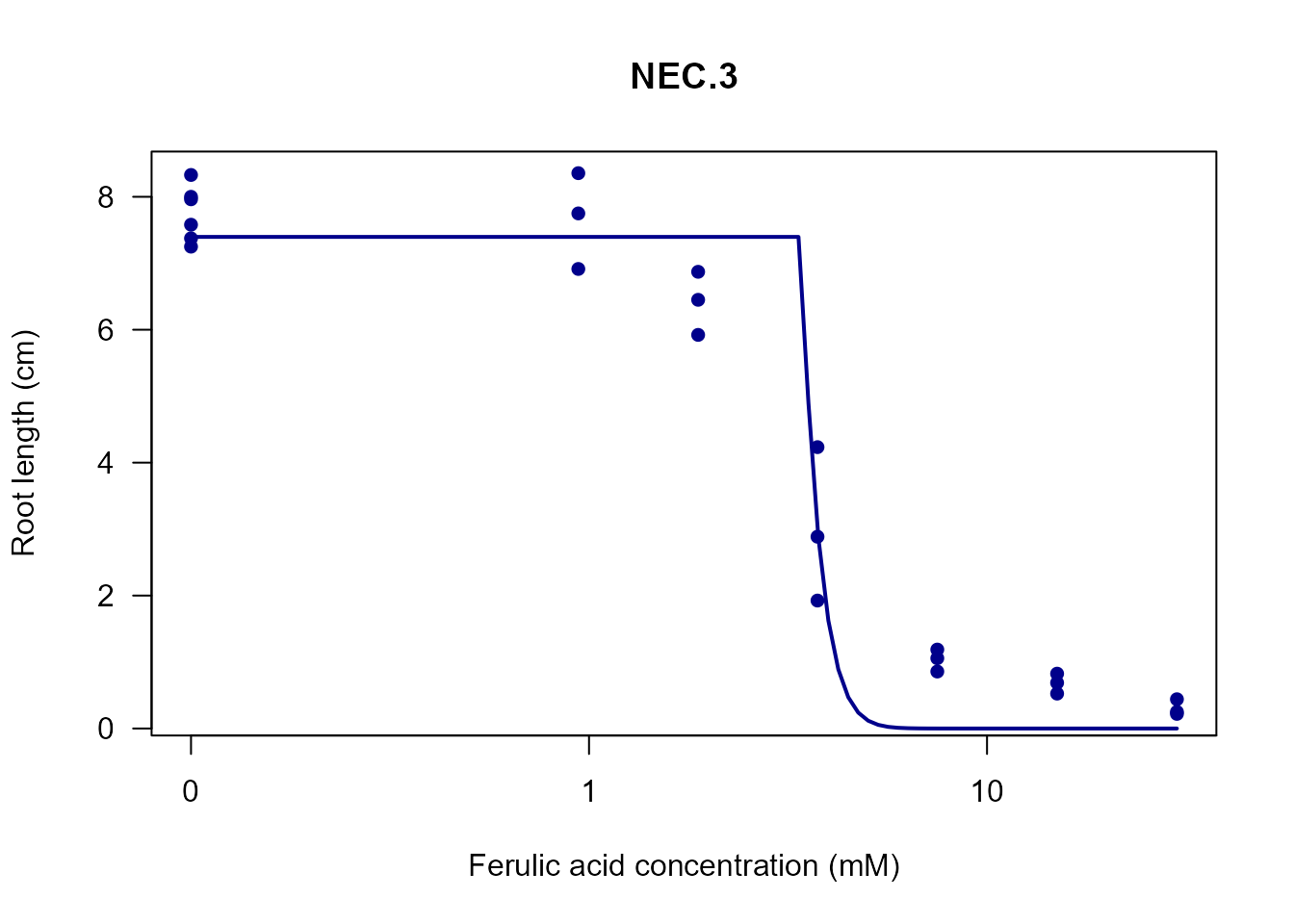

my_plot(nec4.fit, col = "darkred", lwd = 2)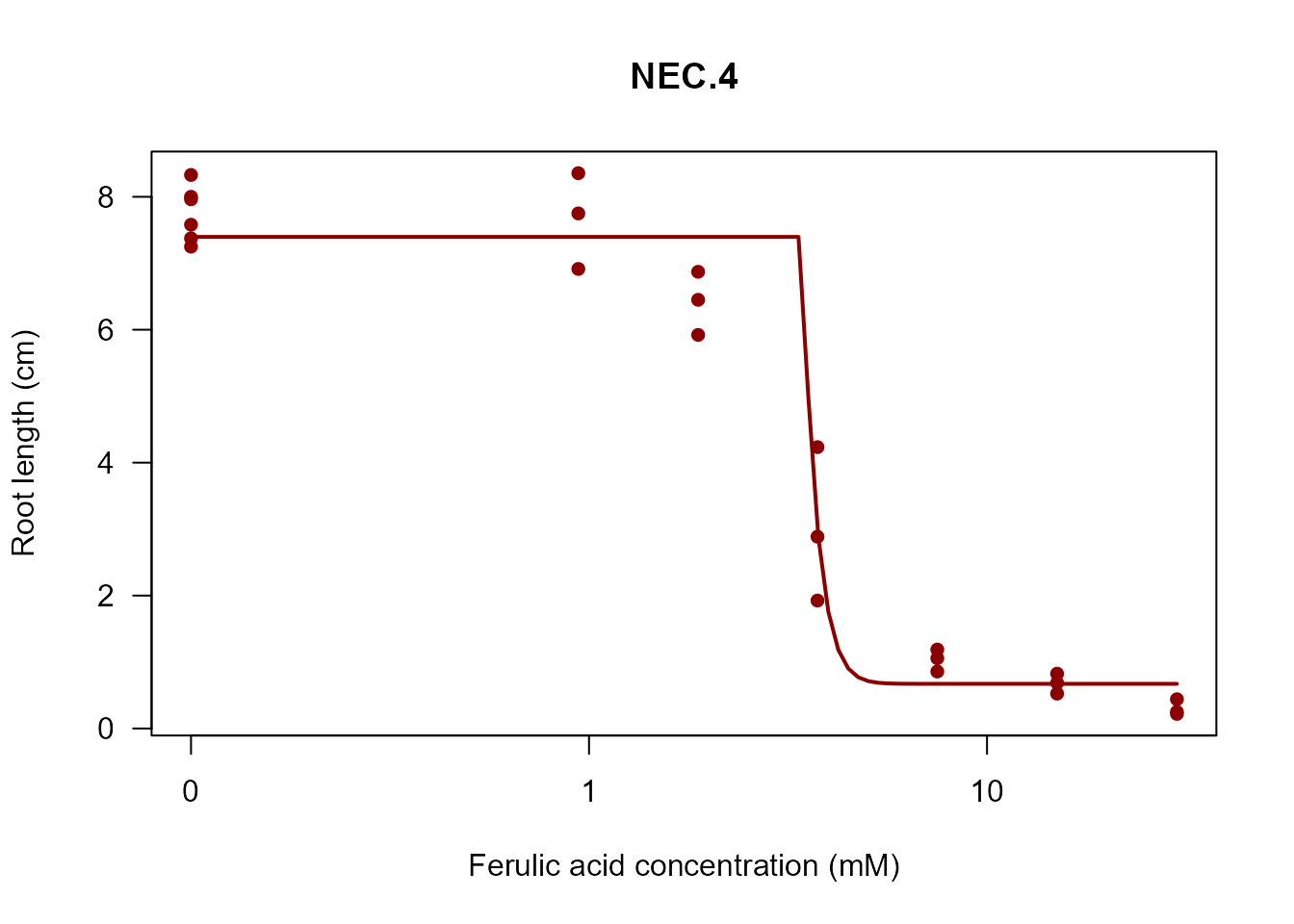

Design Pattern in the drc Package

The NEC functions follow the standard drc package design pattern used consistently across all model families:

Examples of Similar Patterns:

1. Log-logistic models: llogistic, LL.2, LL.3, LL.3u, LL.4, LL.5
2. Weibull type 1: weibull1, W1.2, W1.3, W1.3u, W1.4
3. Weibull type 2: weibull2, W2.2, W2.3, W2.3u, W2.4
4. Gompertz: gompertz, G.2, G.3, G.3u, G.4
5. Log-normal: lnormal, LN.2, LN.3, LN.3u, LN.4

Pattern Structure:

1. Base function (e.g., llogistic, NEC)
   • Provides core implementation with full parameter flexibility
   • Often not exported (used internally)
   • Accepts fixed argument for parameter constraints
2. Numbered variants (e.g., LL.2, LL.3, LL.4, LL.5)
   • Convenience wrappers with common parameter combinations
   • Exported for user convenience
   • Number indicates count of free parameters
   • Each serves specific biological/experimental scenarios

Benefits of This Design:

• User convenience: Common cases are easy to specify
• Parameter identifiability: Constraining parameters when appropriate improves estimation
• Model selection: Easy to compare nested models
• Biological meaning: Parameter constraints reflect experimental knowledge
• Backwards compatibility: Adding variants doesn’t break existing code
• Documentation clarity: Each variant can have specific use-case documentation

Choosing the Right NEC Variant

Here’s a decision guide to help you choose the appropriate NEC function:

1. Do you know both the lower and upper response limits?
   • Yes → Use NEC.2
   • No → Go to step 2
2. Is your baseline (control) response zero or can it be assumed to be zero?
   • Yes → Use NEC.3 (most common case)
   • No → Go to step 3
3. Do you need to estimate all parameters from the data?
   • Yes → Use NEC.4
   • Unsure → Start with NEC.3 and compare with NEC.4 using model selection criteria (AIC, BIC)

Example Decision Process:

# Toxicology study with percentage mortality (0-100%)
# Known bounds: lower = 0%, upper = 100%
# → Use NEC.2
mortality.model <- drm(mortality ~ dose, data = mydata, fct = NEC.2(upper = 100))

# Plant growth study measuring root length
# Control (no treatment) shows some growth (not zero)
# → Try both NEC.3 and NEC.4, compare with AIC
model3 <- drm(rootlength ~ concentration, data = mydata, fct = NEC.3())
model4 <- drm(rootlength ~ concentration, data = mydata, fct = NEC.4())
mselect(model3, model4)

# Standard dose-response with zero baseline
# Maximum response unknown
# → Use NEC.3
response.model <- drm(response ~ dose, data = mydata, fct = NEC.3())

Redundancy Assessment

Are any NEC functions redundant?

Answer: NO - All functions are necessary.

Reasoning:

1. NEC (base function)
   • Cannot be removed: Contains the actual mathematical implementation
   • All other functions are wrappers that call NEC with specific constraints
   • Removing it would break NEC.2, NEC.3, and NEC.4
2. NEC.2
   • Unique purpose: Only variant with both upper and lower limits fixed
   • Distinct use case: Bounded response scales (proportions, percentages)
   • Cannot be replicated: NEC.3 fixes only lower limit, NEC.4 fixes nothing
   • Statistical benefit: Reduces parameters from 4 to 2, greatly improving identifiability
3. NEC.3
   • Most common scenario: Standard toxicology with zero baseline
   • Optimal balance: More flexible than NEC.2, more stable than NEC.4
   • Common convention: Matches typical experimental designs where control = 0
   • Unique constraint: Only variant fixing lower limit while freeing upper limit
4. NEC.4
   • Essential for flexibility: Only way to estimate all 4 parameters
   • Model selection: Needed for comparing against constrained models
   • Non-zero baselines: Only option when control response is unknown and non-zero
   • Diagnostic tool: Helps determine if constraints are appropriate

User Experience Comparison:

If functions were combined, users would need to manually specify constraints:

# Current approach (user-friendly):
drm(y ~ x, data = mydata, fct = NEC.3())

# If combined (cumbersome and error-prone):
drm(y ~ x, data = mydata, fct = NEC(fixed = c(NA, 0, NA, NA)))

The current design: - Reduces usability barriers - Prevents errors from wrong constraint specifications - Provides helpful documentation for common cases - Maintains backwards compatibility - Follows established drc package conventions

Practical Tips

1. Starting with Model Selection

When unsure which variant to use, start with NEC.3 (most common) and compare with other variants:

# Fit an initial model, then compare with alternative NEC variants
m3 <- drm(response ~ dose, data = mydata, fct = NEC.3())

# Compare using model selection (mselect takes one fitted model + a list of alternatives)
mselect(m3, fctList = list(NEC.2(), NEC.4()))

2. Checking Parameter Identifiability

If your NEC.4 model shows very large standard errors or fails to converge, consider constraining parameters:

# If NEC.4 has convergence issues, try NEC.3
summary(nec4.model)  # Check standard errors
# If c is close to 0 with large SE, use NEC.3
nec3.model <- drm(response ~ dose, data = mydata, fct = NEC.3())

3. Interpreting the Threshold Parameter

The e parameter represents the NEC threshold - the concentration below which there is no effect:

# Extract the threshold estimate
threshold <- coef(nec3.model)["e:(Intercept)"]
cat("Estimated NEC threshold:", threshold, "\n")

# Get confidence interval for the threshold
confint(nec3.model)

Conclusion

All 4 NEC functions serve distinct and necessary purposes in the drc package:

• NEC: Internal implementation engine
• NEC.2: Highly constrained models with known bounds (2 parameters)
• NEC.3: Standard case with zero baseline (3 parameters) - most commonly used
• NEC.4: Full flexibility for complex scenarios (4 parameters)

The design represents:

1. Sound software architecture: Internal implementation separated from user interface
2. Statistical best practice: Providing appropriate model complexity for different scenarios
3. User experience optimization: Common cases are simple, complex cases are possible
4. Package consistency: Matches the established pattern used for all other model families

References

Pires, A. M., Branco, J. A., Picado, A., Mendonca, E. (2002) Models for the estimation of a ‘no effect concentration’, Environmetrics, 13, 15-27.

See Also

• ?NEC - Base NEC function documentation
• ?NEC.2 - Two-parameter NEC model
• ?NEC.3 - Three-parameter NEC model
• ?NEC.4 - Four-parameter NEC model
• ?drm - Main function for fitting dose-response models
• ?mselect - Model selection function