Potency of two herbicides

Data are from an experiment, comparing the potency of the two herbicides glyphosate and bentazone in white mustard Sinapis alba.

Usage

data(S.alba.comp)

Format

A data frame with 141 observations on the following 8 variables.

exp

a factor with levels ben1, ben2, gly1, gly2 indicating which experiment each observation belongs to.

herbicide

a factor with levels Bentazone Glyphosate (the two herbicides applied).

dose

a numeric vector containing the dose in g/ha.

drymatter

a numeric vector containing the response (dry matter in g/pot).

Tf

a numeric vector .

area

a numeric vector .

Fo

a numeric vector .

Fm

a numeric vector .

Details

The lower and upper limits for the two herbicides can be assumed identical, whereas slopes and ED50 values are different (in the log-logistic model).

Source

Christensen, M. G. and Teicher, H. B., and Streibig, J. C. (2003) Linking fluorescence induction curve and biomass in herbicide screening, Pest Management Science, 59, 1303–1310.

Examples

library(drc)

## Displaying the data
head(S.alba.comp)
#>    exp herbicide dose drymatter  Tf  area  Fo   Fm
#> 1 ben1 bentazone    0       4.1 200 31200 278 1662
#> 2 ben1 bentazone    0       3.4 230 30600 278 1670
#> 3 ben1 bentazone    0       2.6 210 27400 299 1646
#> 4 ben1 bentazone    0       3.5 260 34600 288 1715
#> 5 ben1 bentazone    0       4.3 200 31000 272 1651
#> 6 ben1 bentazone    0       4.2 240 31400 286 1681

## Fitting a four-parameter log-logistic model with common upper and lower limits
S.alba.comp.m1 <- drm(drymatter ~ dose, herbicide, data = S.alba.comp, fct = LL.4(),
pmodels = list(~herbicide, ~1, ~1, ~herbicide))
summary(S.alba.comp.m1)
#> 
#> Model fitted: Log-logistic (ED50 as parameter) (4 parms)
#> 
#> Parameter estimates:
#> 
#>                        Estimate Std. Error t-value   p-value    
#> b:(Intercept)          5.036275   2.100683  2.3974   0.01788 *  
#> b:herbicideglyphosate -3.682298   2.062582 -1.7853   0.07646 .  
#> c:(Intercept)          0.734059   0.081999  8.9520 2.432e-15 ***
#> d:(Intercept)          3.962500   0.079820 49.6428 < 2.2e-16 ***
#> e:(Intercept)         21.060041   1.286127 16.3748 < 2.2e-16 ***
#> e:herbicideglyphosate 27.165817   5.568005  4.8789 2.958e-06 ***
#> ---
#> Signif. codes:  0 '***' 0.001 '**' 0.01 '*' 0.05 '.' 0.1 ' ' 1
#> 
#> Residual standard error:
#> 
#>  0.495335 (135 degrees of freedom)

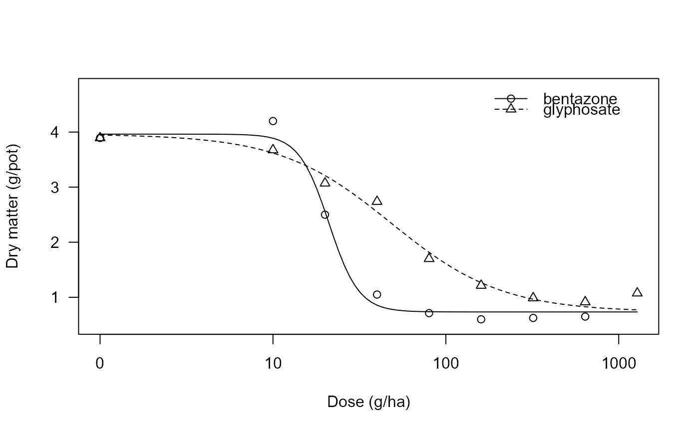
## Plotting the fitted curves
plot(S.alba.comp.m1, xlab = "Dose (g/ha)", ylab = "Dry matter (g/pot)")