Effect of cadmium on growth of green alga
S.capricornutum.RdGreen alga (Selenastrum capricornutum) was exposed to cadmium chloride concentrations ranging from 5 to 80 micro g/L in geometric progression in 4-day population growth test.
Usage
data(S.capricornutum)Format
A data frame with 18 observations on the following 2 variables.
conca numeric vector of cadmium chloride concentrations (micro g/L)
counta numeric vector of algal counts (10000 x cells /ml)
Details
The data are analysed in Bruce and Versteeg (1992) using a log-normal dose-response model (using the logarithm with base 10).
Source
Bruce, R. D. and Versteeg, D. J. (1992) A statistical procedure for modeling continuous toxicity data, Environ. Toxicol. Chem., 11, 1485–1494.
Examples
library(drc)
## Fitting 3-parameter log-normal model
s.cap.m1 <- drm(count ~ conc, data = S.capricornutum, fct = LN.3())
## Residual plot
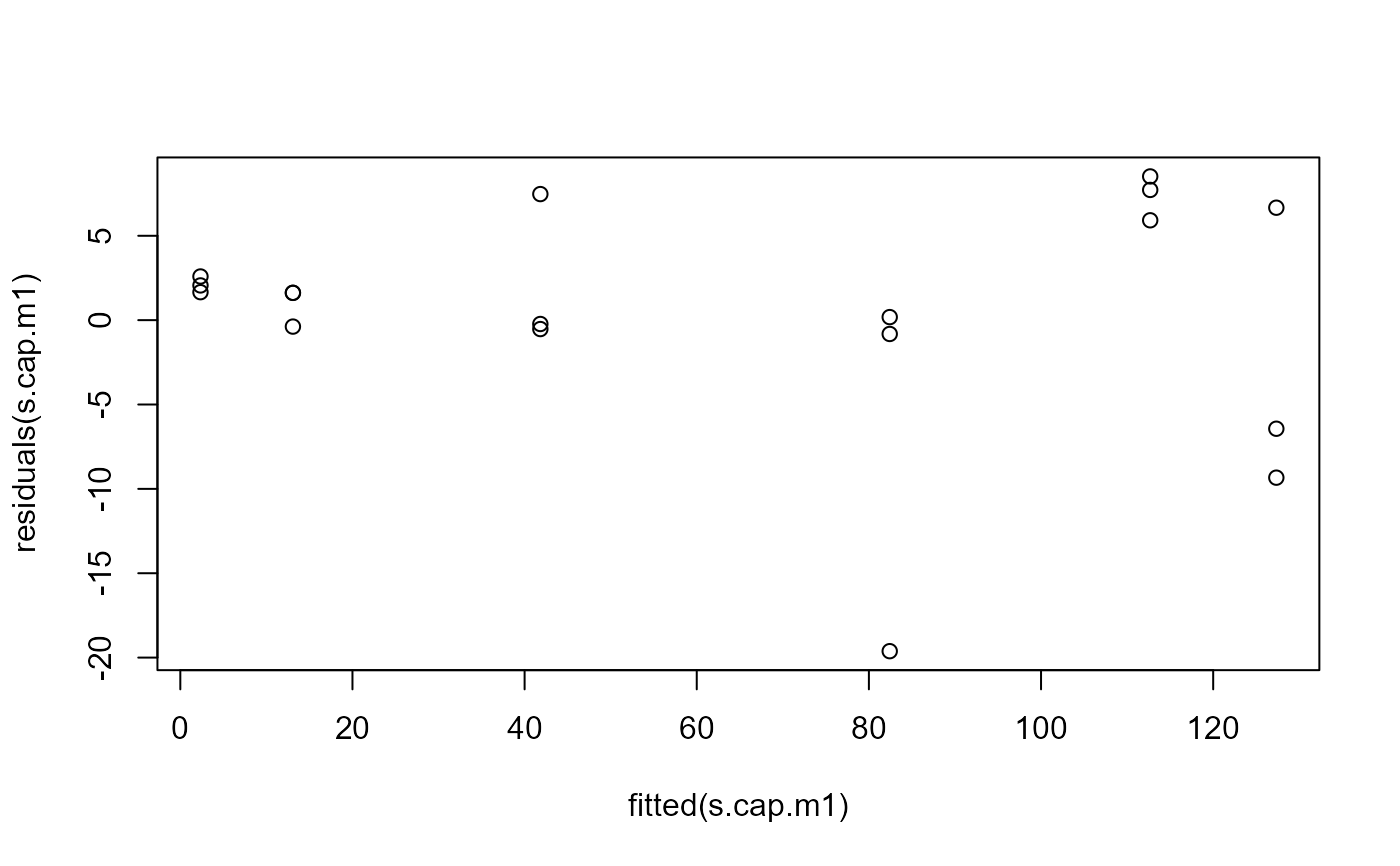
plot(fitted(s.cap.m1), residuals(s.cap.m1))
 ## Fitting model with transform-both-sides approach
s.cap.m2 <- boxcox(s.cap.m1, method = "anova")
## Fitting model with transform-both-sides approach
s.cap.m2 <- boxcox(s.cap.m1, method = "anova")
 summary(s.cap.m2)
#>
#> Model fitted: Log-normal with lower limit at 0 (3 parms)
#>
#> Parameter estimates:
#>
#> Estimate Std. Error t-value p-value
#> b:(Intercept) -1.000982 0.044845 -22.321 6.394e-13 ***
#> d:(Intercept) 132.079098 7.554011 17.485 2.191e-11 ***
#> e:(Intercept) 12.428164 1.100916 11.289 9.915e-09 ***
#> ---
#> Signif. codes: 0 '***' 0.001 '**' 0.01 '*' 0.05 '.' 0.1 ' ' 1
#>
#> Residual standard error:
#>
#> 0.1551479 (15 degrees of freedom)
#>
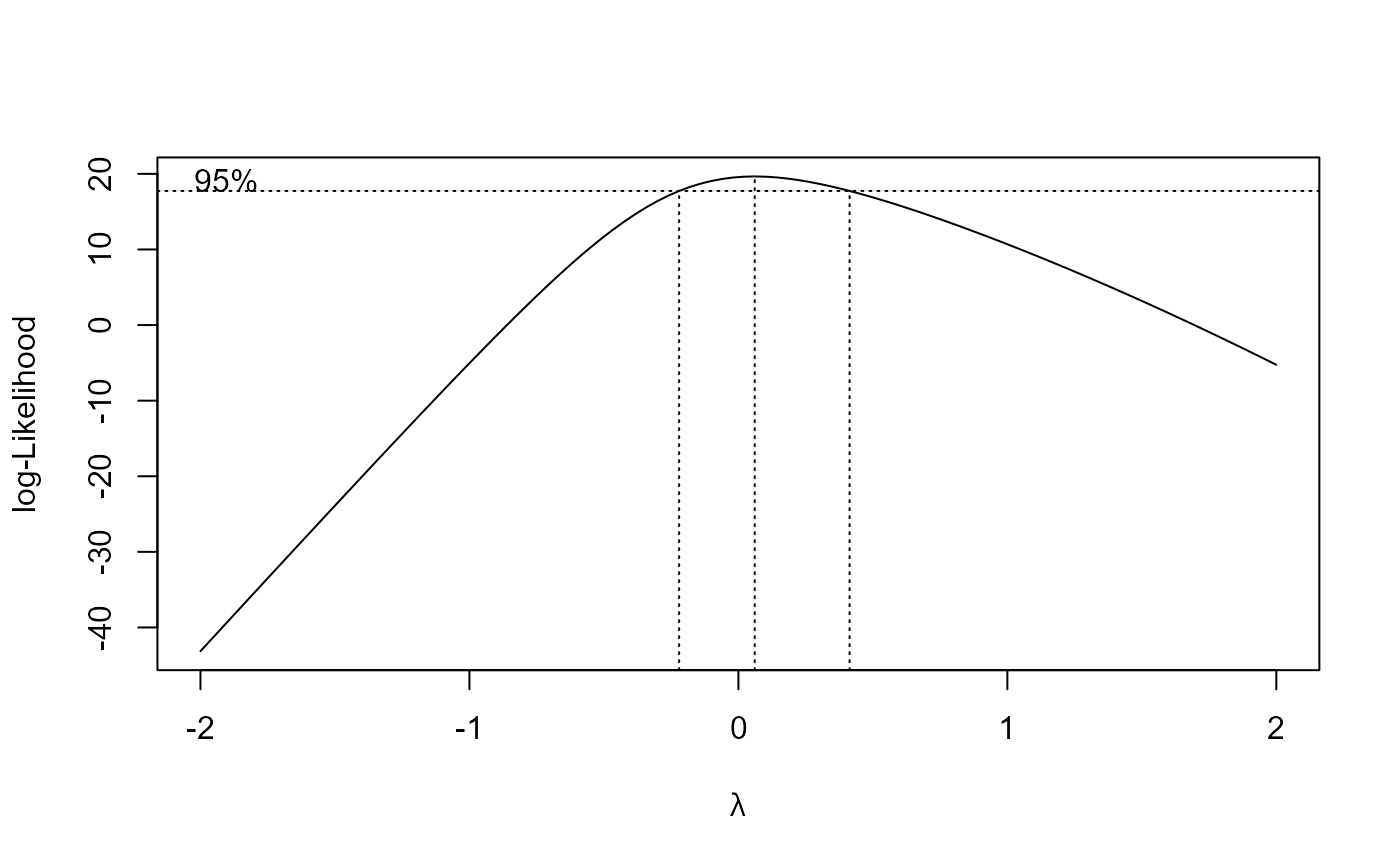
#> Non-normality/heterogeneity adjustment through Box-Cox transformation
#>
#> Estimated lambda: 0.0606
#> Confidence interval for lambda: [-0.220, 0.414]
#>
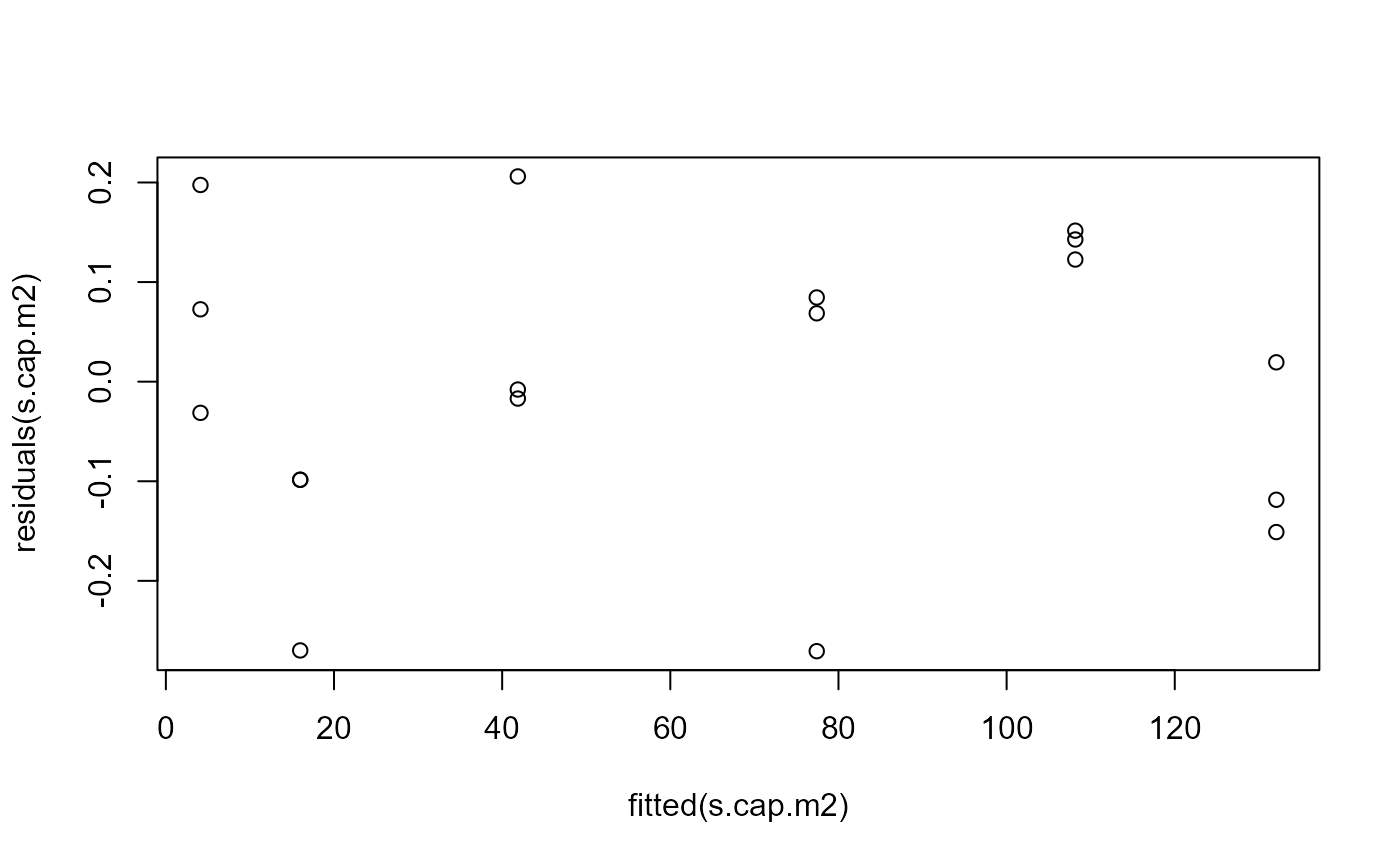
## Residual plot after transformation (looks better)
plot(fitted(s.cap.m2), residuals(s.cap.m2))
summary(s.cap.m2)
#>
#> Model fitted: Log-normal with lower limit at 0 (3 parms)
#>
#> Parameter estimates:
#>
#> Estimate Std. Error t-value p-value
#> b:(Intercept) -1.000982 0.044845 -22.321 6.394e-13 ***
#> d:(Intercept) 132.079098 7.554011 17.485 2.191e-11 ***
#> e:(Intercept) 12.428164 1.100916 11.289 9.915e-09 ***
#> ---
#> Signif. codes: 0 '***' 0.001 '**' 0.01 '*' 0.05 '.' 0.1 ' ' 1
#>
#> Residual standard error:
#>
#> 0.1551479 (15 degrees of freedom)
#>
#> Non-normality/heterogeneity adjustment through Box-Cox transformation
#>
#> Estimated lambda: 0.0606
#> Confidence interval for lambda: [-0.220, 0.414]
#>
## Residual plot after transformation (looks better)
plot(fitted(s.cap.m2), residuals(s.cap.m2))
 ## Calculating ED values on log scale
ED(s.cap.m2, c(10, 20, 50), interval="delta")
#>
#> Estimated effective doses
#>
#> Estimate Std. Error Lower Upper
#> e:10 3.45448 0.49164 2.40656 4.50239
#> e:20 5.36110 0.66213 3.94980 6.77241
#> e:50 12.42816 1.10092 10.08162 14.77471
## Fitting model with ED50 as parameter
## (for comparison)
s.cap.m3 <- drm(count ~ conc, data = S.capricornutum, fct = LN.3(loge=TRUE))
s.cap.m4 <- boxcox(s.cap.m3, method = "anova")
## Calculating ED values on log scale
ED(s.cap.m2, c(10, 20, 50), interval="delta")
#>
#> Estimated effective doses
#>
#> Estimate Std. Error Lower Upper
#> e:10 3.45448 0.49164 2.40656 4.50239
#> e:20 5.36110 0.66213 3.94980 6.77241
#> e:50 12.42816 1.10092 10.08162 14.77471
## Fitting model with ED50 as parameter
## (for comparison)
s.cap.m3 <- drm(count ~ conc, data = S.capricornutum, fct = LN.3(loge=TRUE))
s.cap.m4 <- boxcox(s.cap.m3, method = "anova")
 summary(s.cap.m4)
#>
#> Model fitted: Log-normal with lower limit at 0 (3 parms)
#>
#> Parameter estimates:
#>
#> Estimate Std. Error t-value p-value
#> b:(Intercept) -1.000991 0.044846 -22.320 6.395e-13 ***
#> d:(Intercept) 132.078306 7.553934 17.485 2.191e-11 ***
#> e:(Intercept) 2.519975 0.088583 28.448 1.821e-14 ***
#> ---
#> Signif. codes: 0 '***' 0.001 '**' 0.01 '*' 0.05 '.' 0.1 ' ' 1
#>
#> Residual standard error:
#>
#> 0.1551479 (15 degrees of freedom)
#>
#> Non-normality/heterogeneity adjustment through Box-Cox transformation
#>
#> Estimated lambda: 0.0606
#> Confidence interval for lambda: [-0.220, 0.414]
#>
ED(s.cap.m4, c(10, 20, 50), interval = "fls")
#>
#> Estimated effective doses
#>
#> Estimate Std. Error Lower Upper
#> e:10 3.454549 0.142322 2.550630 4.678808
#> e:20 5.361195 0.123508 4.120343 6.975731
#> e:50 12.428289 0.088583 10.289930 15.011022
summary(s.cap.m4)
#>
#> Model fitted: Log-normal with lower limit at 0 (3 parms)
#>
#> Parameter estimates:
#>
#> Estimate Std. Error t-value p-value
#> b:(Intercept) -1.000991 0.044846 -22.320 6.395e-13 ***
#> d:(Intercept) 132.078306 7.553934 17.485 2.191e-11 ***
#> e:(Intercept) 2.519975 0.088583 28.448 1.821e-14 ***
#> ---
#> Signif. codes: 0 '***' 0.001 '**' 0.01 '*' 0.05 '.' 0.1 ' ' 1
#>
#> Residual standard error:
#>
#> 0.1551479 (15 degrees of freedom)
#>
#> Non-normality/heterogeneity adjustment through Box-Cox transformation
#>
#> Estimated lambda: 0.0606
#> Confidence interval for lambda: [-0.220, 0.414]
#>
ED(s.cap.m4, c(10, 20, 50), interval = "fls")
#>
#> Estimated effective doses
#>
#> Estimate Std. Error Lower Upper
#> e:10 3.454549 0.142322 2.550630 4.678808
#> e:20 5.361195 0.123508 4.120343 6.975731
#> e:50 12.428289 0.088583 10.289930 15.011022