Finds the optimal Box-Cox transformation for non-linear regression.
Usage
# S3 method for class 'drc'
boxcox(
  object,
  lambda = seq(-2, 2, by = 0.25),
  plotit = TRUE,
  bcAdd = 0,
  method = c("ml", "anova"),
  level = 0.95,
  eps = 1/50,
  xlab = expression(lambda),
  ylab = "log-Likelihood",
  ...
)
Arguments
- object
object of class
drc.- lambda
numeric vector of lambda values; the default is (-2, 2) in steps of 0.25.
- plotit
logical which controls whether the result should be plotted.
- bcAdd
numeric value specifying the constant to be added on both sides prior to Box-Cox transformation. The default is 0.
- method
character string specifying the estimation method for lambda: maximum likelihood or ANOVA-based (optimal lambda inherited from more general ANOVA model fit).
- level
numeric value: the confidence level required.
- eps
numeric value: the tolerance for lambda = 0; defaults to 0.02.
- xlab
character string: the label on the x axis, defaults to "lambda".
- ylab
character string: the label on the y axis, defaults to "log-likelihood".
- ...
additional graphical parameters.
Value
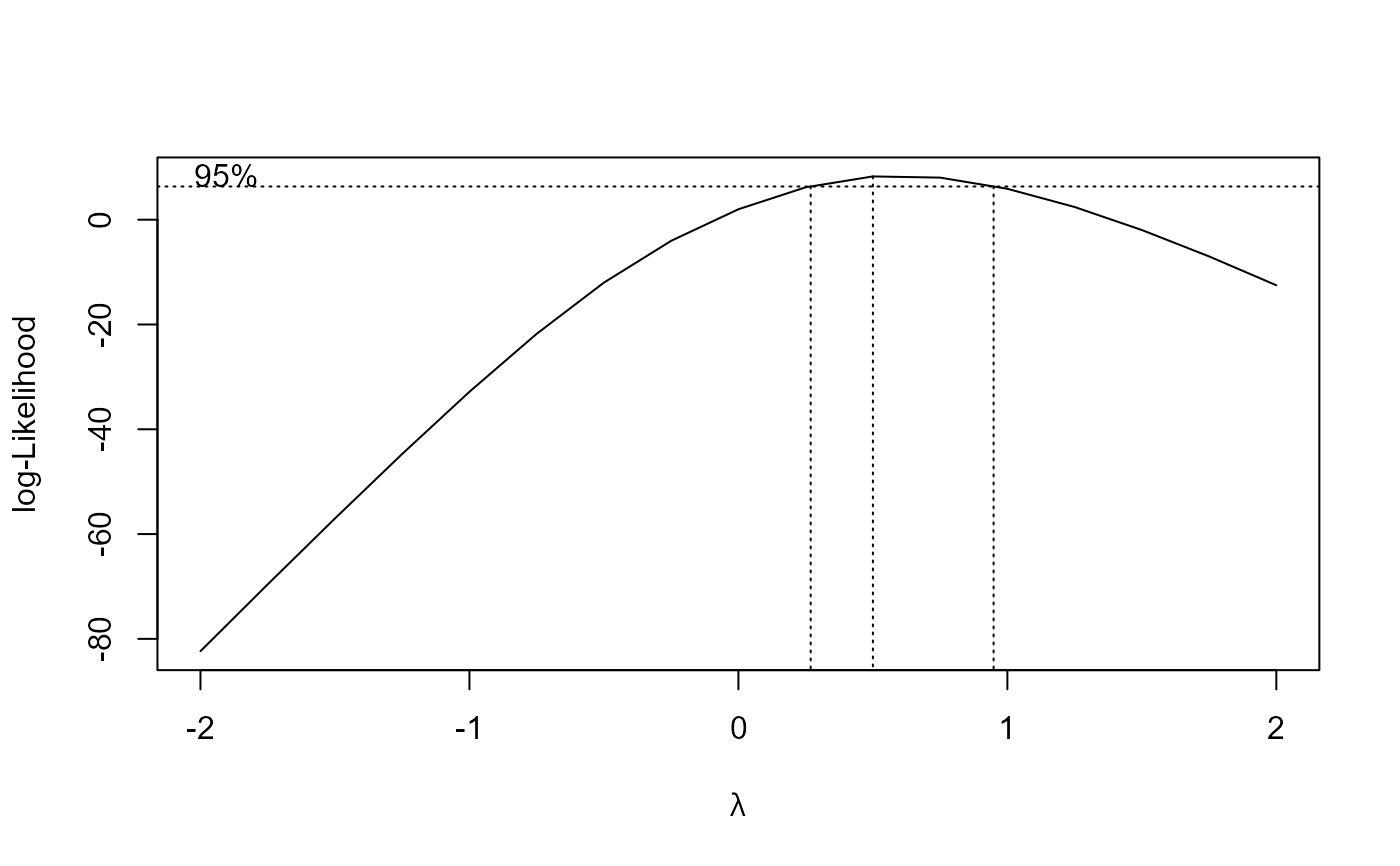
An object of class "drc" (returned invisibly). If plotit = TRUE a plot of loglik vs lambda is shown indicating a confidence interval (by default 95%) about the optimal lambda value.
Details
The optimal lambda value is determined using a profile likelihood approach: For each lambda value the dose-response regression model is fitted and the lambda value (and corresponding model fit) resulting in the largest value of the log likelihood function is chosen.
References
Carroll, R. J. and Ruppert, D. (1988) Transformation and Weighting in Regression, New York: Chapman and Hall (Chapter 4).
See also
For linear regression the analogue is boxcox.
Examples
## Fitting log-logistic model without transformation
ryegrass.m1 <- drm(ryegrass, fct = LL.4())
summary(ryegrass.m1)
#>
#> Model fitted: Log-logistic (ED50 as parameter) (4 parms)
#>
#> Parameter estimates:
#>
#>               Estimate Std. Error t-value   p-value
#> b:(Intercept)  2.98222    0.46506  6.4125 2.960e-06 ***
#> c:(Intercept)  0.48141    0.21219  2.2688   0.03451 *
#> d:(Intercept)  7.79296    0.18857 41.3272 < 2.2e-16 ***
#> e:(Intercept)  3.05795    0.18573 16.4644 4.268e-13 ***
#> ---
#> Signif. codes:  0 '***' 0.001 '**' 0.01 '*' 0.05 '.' 0.1 ' ' 1
#>
#> Residual standard error:
#>
#>  0.5196256 (20 degrees of freedom)

## Fitting the same model with the optimal Box-Cox transformation
ryegrass.m2 <- boxcox(ryegrass.m1)

summary(ryegrass.m2)
#>
#> Model fitted: Log-logistic (ED50 as parameter) (4 parms)
#>
#> Parameter estimates:
#>
#>               Estimate Std. Error t-value   p-value
#> b:(Intercept)  2.61839    0.39151  6.6880 1.649e-06 ***
#> c:(Intercept)  0.39083    0.10429  3.7474  0.001269 **
#> d:(Intercept)  7.86633    0.29558 26.6136 < 2.2e-16 ***
#> e:(Intercept)  3.01662    0.21005 14.3612 5.354e-12 ***
#> ---
#> Signif. codes:  0 '***' 0.001 '**' 0.01 '*' 0.05 '.' 0.1 ' ' 1
#>
#> Residual standard error:
#>
#>  0.2962958 (20 degrees of freedom)
#>
#> Non-normality/heterogeneity adjustment through Box-Cox transformation
#>
#> Estimated lambda: 0.5
#> Confidence interval for lambda: [0.269,0.949]
#>
summary(ryegrass.m2)
#>
#> Model fitted: Log-logistic (ED50 as parameter) (4 parms)
#>
#> Parameter estimates:
#>
#> Estimate Std. Error t-value p-value
#> b:(Intercept) 2.61839 0.39151 6.6880 1.649e-06 ***
#> c:(Intercept) 0.39083 0.10429 3.7474 0.001269 **
#> d:(Intercept) 7.86633 0.29558 26.6136 < 2.2e-16 ***
#> e:(Intercept) 3.01662 0.21005 14.3612 5.354e-12 ***
#> ---
#> Signif. codes: 0 '***' 0.001 '**' 0.01 '*' 0.05 '.' 0.1 ' ' 1
#>
#> Residual standard error:
#>
#> 0.2962958 (20 degrees of freedom)
#>
#> Non-normality/heterogeneity adjustment through Box-Cox transformation
#>
#> Estimated lambda: 0.5
#> Confidence interval for lambda: [0.269,0.949]
#>