Daphnia test — daphnids • drc

The number of immobile daphnids –in contrast to mobile daphnids– out of a total of 20 daphnids was counted for several concentrations of a toxic substance.

Usage

data(daphnids)

Format

A data frame with 16 observations on the following 4 variables.

dose: a numeric vector
no: a numeric vector
total: a numeric vector
time: a factor with levels 24h 48h

Details

The same daphnids were counted at 24h and later again at 48h.

Source

Nina Cedergreen, Faculty of Life Sciences, University of Copenhagen, Denmark.

Examples

library(drc)

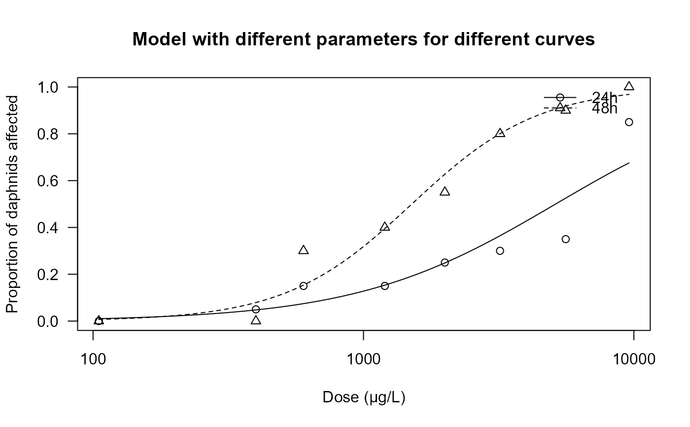
## Fitting a model with different parameters
## for different curves
daphnids.m1 <- drm( data = daphnids, no/total~dose, 
                    curveid = time, weights = total, 
                    fct = LL.2(), type = "binomial" )

## plot models
plot(daphnids.m1, ylim = c(0, 1),
     xlab = "Dose (µg/L)", ylab = "Proportion of daphnids affected", 
     main = "Model with different parameters for different curves")


## Goodness-of-fit test
modelFit(daphnids.m1)
#> Goodness-of-fit test
#> 
#>             Df Chisq value p value
#>                                   
#> DRC model   12      13.873  0.3089

## Summary of the data
summary(daphnids.m1)
#> 
#> Model fitted: Log-logistic (ED50 as parameter) with lower limit at 0 and upper limit at 1 (2 parms)
#> 
#> Parameter estimates:
#> 
#>         Estimate Std. Error t-value   p-value    
#> b:24h   -1.17384    0.22236 -5.2791 1.298e-07 ***
#> b:48h   -1.84968    0.27922 -6.6244 3.488e-11 ***
#> e:24h 5134.03344 1056.74197  4.8584 1.184e-06 ***
#> e:48h 1509.06539  187.76008  8.0372 9.037e-16 ***
#> ---
#> Signif. codes:  0 '***' 0.001 '**' 0.01 '*' 0.05 '.' 0.1 ' ' 1

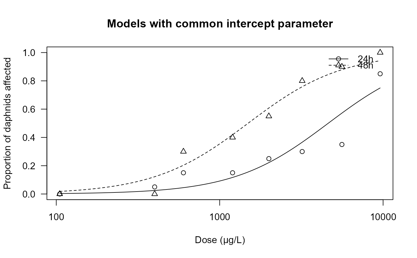
## Fitting a model with a common intercept parameter
daphnids.m2 <- drm(no/total~dose, curveid = time, weights = total, 
                   data = daphnids, fct = LL.2(), type = "binomial", 
                   pmodels = list(~1, ~time))

## plot models
plot(daphnids.m2, ylim = c(0, 1),
     xlab = "Dose (µg/L)", ylab = "Proportion of daphnids affected", 
     main = "Models with common intercept parameter")


## Goodness-of-fit test
modelFit(daphnids.m2)
#> Goodness-of-fit test
#> 
#>             Df Chisq value p value
#>                                   
#> DRC model   13       17.63  0.1721

## Summary of the data
summary(daphnids.m2)
#> 
#> Model fitted: Log-logistic (ED50 as parameter) with lower limit at 0 and upper limit at 1 (2 parms)
#> 
#> Parameter estimates:
#> 
#>                  Estimate  Std. Error t-value   p-value    
#> b:(Intercept)    -1.49926     0.17345 -8.6436 < 2.2e-16 ***
#> e:(Intercept)  4614.39264   708.09425  6.5166 7.190e-11 ***
#> e:time48h     -3122.47346   741.26254 -4.2124 2.527e-05 ***
#> ---
#> Signif. codes:  0 '***' 0.001 '**' 0.01 '*' 0.05 '.' 0.1 ' ' 1