Deguelin applied to chrysanthemum aphis

Quantal assay data from an experiment where the insectide deguelin was applied to Macrosiphoniella sanborni.

Usage

data(deguelin)

Format

A data frame with 6 observations on the following 4 variables.

dose: a numeric vector of doses applied
log10dose: a numeric vector of logarithm-transformed doses
r: a numeric vector contained number of dead insects
n: a numeric vector contained the total number of insects

Details

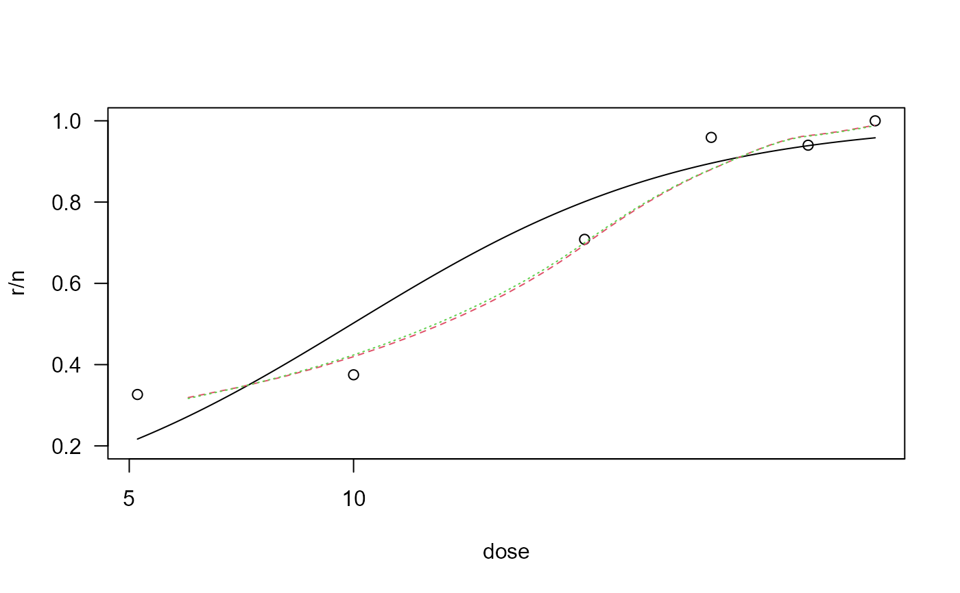
The log-logistic model provides an inadequate fit.

The dataset is used in Nottingham and Birch (2000) to illustrate a semiparametric approach to dose-response modelling.

Source

Morgan, B. J. T. (1992) Analysis of Quantal Response Data, London: Chapman & Hall/CRC (Table 3.9, p. 117).

References

Notttingham, Q. J. and Birch, J. B. (2000) A semiparametric approach to analysing dose-response data, Statist. Med., 19, 389–404.

Examples

library(drc)

## Log-logistic fit
deguelin.m1 <- drm(r/n~dose, weights=n, data=deguelin, fct=LL.2(), type="binomial")
modelFit(deguelin.m1)
#> Goodness-of-fit test
#> 
#>             Df Chisq value p value
#>                                   
#> DRC model    4      13.375  0.0096
summary(deguelin.m1)
#> 
#> Model fitted: Log-logistic (ED50 as parameter) with lower limit at 0 and upper limit at 1 (2 parms)
#> 
#> Parameter estimates:
#> 
#>               Estimate Std. Error t-value   p-value    
#> b:(Intercept) -1.93709    0.22390 -8.6514 < 2.2e-16 ***
#> e:(Intercept)  9.95219    0.92186 10.7958 < 2.2e-16 ***
#> ---
#> Signif. codes:  0 '***' 0.001 '**' 0.01 '*' 0.05 '.' 0.1 ' ' 1

## Loess fit
deguelin.m2 <- loess(r/n~dose, data=deguelin, degree=1)

## Plot of data with fits superimposed
plot(deguelin.m1, ylim=c(0.2,1))
lines(1:60, predict(deguelin.m2, newdata=data.frame(dose=1:60)), col = 2, lty = 2)

lines(1:60, 0.95*predict(deguelin.m2, 
newdata=data.frame(dose=1:60))+0.05*predict(deguelin.m1, newdata=data.frame(dose=1:60), se = FALSE),
col = 3, lty=3)