Effect of erythromycin on mixed sewage microorganisms
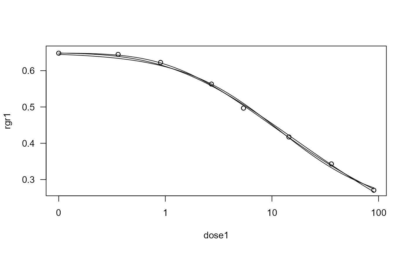
etmotc.RdRelative growth rate in biomass of mixed sewage microorganisms (per hour) as a function of increasing concentrations of the antibiotic erythromycin (mg/l).
Usage
data(etmotc)Format
A data frame with 57 observations on the following 4 variables.
cella numeric vector
dose1a numeric vector
pct1a numeric vector
rgr1a numeric vector
Details
Data stem from an experiment investigating the effect of pharmaceuticals, that are used in human and veterinary medicine and that are being released into the aquatic environment through waste water or through manure used for fertilising agricultural land. The experiment constitutes a typical dose-response situation. The dose is concentration of the antibiotic erythromycin (mg/l), which is an antibiotic that can be used by persons or animals showing allergy to penicillin, and the measured response is the relative growth rate in biomass of mixed sewage microorganisms (per hour), measured as turbidity two hours after exposure by means of a spectrophotometer. The experiment was designed in such a way that eight replicates were assigned to the control (dose 0), but no replicates were assigned to the 7 non-zero doses. Further details are found in Christensen et al (2006).
Source
Christensen, A. M. and Ingerslev, F. and Baun, A. 2006 Ecotoxicity of mixtures of antibiotics used in aquacultures, Environmental Toxicology and Chemistry, 25, 2208–2215.
Examples
library(drc)

etmotc.m1<-drm(rgr1~dose1, data=etmotc[1:15,], fct=LL.4())
plot(etmotc.m1)
modelFit(etmotc.m1)
#> Lack-of-fit test
#>
#>           ModelDf       RSS Df F value p value
#> ANOVA           7 5.413e-05
#> DRC model      11 5.978e-04  4 17.5773  0.0009
summary(etmotc.m1)
#>
#> Model fitted: Log-logistic (ED50 as parameter) (4 parms)
#>
#> Parameter estimates:
#>
#>                 Estimate Std. Error  t-value   p-value
#> b:(Intercept)  0.9365452  0.0680380  13.7650 2.806e-08 ***
#> c:(Intercept)  0.2225885  0.0199342  11.1662 2.430e-07 ***
#> d:(Intercept)  0.6496673  0.0025117 258.6611 < 2.2e-16 ***
#> e:(Intercept) 11.6675539  1.6207593   7.1988 1.755e-05 ***
#> ---
#> Signif. codes:  0 '***' 0.001 '**' 0.01 '*' 0.05 '.' 0.1 ' ' 1
#>
#> Residual standard error:
#>
#>  0.007371964 (11 degrees of freedom)

etmotc.m2<-drm(rgr1~dose1, data=etmotc[1:15,], fct=W2.4())
plot(etmotc.m2, add = TRUE)
modelFit(etmotc.m2)
#> Lack-of-fit test
#>
#>           ModelDf        RSS Df F value p value
#> ANOVA           7 5.4128e-05
#> DRC model      11 1.5608e-04  4  3.2960  0.0807
summary(etmotc.m2)
#>
#> Model fitted: Weibull (type 2) (4 parms)
#>
#> Parameter estimates:
#>
#>                 Estimate Std. Error  t-value   p-value
#> b:(Intercept) -0.4585014  0.0270713 -16.9368 3.154e-09 ***
#> c:(Intercept)  0.1105817  0.0253882   4.3556  0.001145 **
#> d:(Intercept)  0.6484347  0.0012874 503.6837 < 2.2e-16 ***
#> e:(Intercept)  9.8112667  1.1944769   8.2139 5.079e-06 ***
#> ---
#> Signif. codes:  0 '***' 0.001 '**' 0.01 '*' 0.05 '.' 0.1 ' ' 1
#>
#> Residual standard error:
#>
#>  0.003766782 (11 degrees of freedom)

etmotc.m3<-drm(rgr1~dose1, data=etmotc[1:15,], fct=W2.3())
plot(etmotc.m3, add = TRUE)

modelFit(etmotc.m3)
#> Lack-of-fit test
#>
#>           ModelDf        RSS Df F value p value
#> ANOVA           7 5.4128e-05
#> DRC model      12 3.0527e-04  5  6.4955  0.0146
summary(etmotc.m3)
#>
#> Model fitted: Weibull (type 2) with lower limit at 0 (3 parms)
#>
#> Parameter estimates:
#>
#>                 Estimate Std. Error t-value   p-value
#> b:(Intercept) -0.3748065  0.0079192 -47.329 5.252e-15 ***
#> d:(Intercept)  0.6491863  0.0017073 380.232 < 2.2e-16 ***
#> e:(Intercept) 16.3999632  0.5104155  32.131 5.217e-13 ***
#> ---
#> Signif. codes:  0 '***' 0.001 '**' 0.01 '*' 0.05 '.' 0.1 ' ' 1
#>
#> Residual standard error:
#>
#>  0.005043693 (12 degrees of freedom)
modelFit(etmotc.m3)
#> Lack-of-fit test
#>
#> ModelDf RSS Df F value p value
#> ANOVA 7 5.4128e-05
#> DRC model 12 3.0527e-04 5 6.4955 0.0146
summary(etmotc.m3)
#>
#> Model fitted: Weibull (type 2) with lower limit at 0 (3 parms)
#>
#> Parameter estimates:
#>
#> Estimate Std. Error t-value p-value
#> b:(Intercept) -0.3748065 0.0079192 -47.329 5.252e-15 ***
#> d:(Intercept) 0.6491863 0.0017073 380.232 < 2.2e-16 ***
#> e:(Intercept) 16.3999632 0.5104155 32.131 5.217e-13 ***
#> ---
#> Signif. codes: 0 '***' 0.001 '**' 0.01 '*' 0.05 '.' 0.1 ' ' 1
#>
#> Residual standard error:
#>
#> 0.005043693 (12 degrees of freedom)