Glyphosate and metsulfuron-methyl tested on algae.
glymet.RdThe dataset has 7 mixtures, 8 dilutions, two replicates and 5 common control controls. Four observations are missing, giving a total of 113 observations.
Usage
data(glymet)Format
A data frame with 113 observations on the following 3 variables.
dosea numeric vector of dose values
pcta numeric vector denoting the grouping according to the mixtures percentages
rgra numeric vector of response values (relative growth rates)
Details
The dataset is analysed in Soerensen et al (2007). The concentration addition model can be entertained for this dataset.
Source
The dataset is kindly provided by Nina Cedergreen, Department of Agricultural Sciences, Royal Veterinary and Agricultural University, Denmark.
References
Soerensen, H. and Cedergreen, N. and Skovgaard, I. M. and Streibig, J. C. (2007) An isobole-based statistical model and test for synergism/antagonism in binary mixture toxicity experiments, Environmental and Ecological Statistics, 14, 383–397.
Examples
library(drc)
## Fitting the model with freely varying ED50 values
glymet.free <- drm(rgr~dose, pct, data = glymet,
fct = LL.3(), pmodels = list(~factor(pct) , ~1, ~factor(pct)))
#> Control measurements detected for level: 999
## Lack-of-fit test
modelFit(glymet.free) # acceptable
#> Lack-of-fit test
#>
#> ModelDf RSS Df F value p value
#> ANOVA 57 0.65695
#> DRC model 98 1.35177 41 1.4704 0.0885
summary(glymet.free)
#>
#> Model fitted: Log-logistic (ED50 as parameter) with lower limit at 0 (3 parms)
#>
#> Parameter estimates:
#>
#> Estimate Std. Error t-value p-value
#> b:100 1.6452e+00 2.0683e-01 7.9547 3.169e-12 ***
#> b:83 1.8276e+00 2.3584e-01 7.7492 8.663e-12 ***
#> b:67 1.0654e+00 1.1840e-01 8.9983 1.812e-14 ***
#> b:50 1.2324e+00 1.4031e-01 8.7834 5.262e-14 ***
#> b:33 1.3676e+00 1.6478e-01 8.2992 5.809e-13 ***
#> b:17 1.0100e+00 1.2156e-01 8.3090 5.534e-13 ***
#> b:0 7.1041e-01 9.2251e-02 7.7008 1.097e-11 ***
#> d:(Intercept) 1.6191e+00 2.5370e-02 63.8198 < 2.2e-16 ***
#> e:100 1.3332e+05 1.1477e+04 11.6158 < 2.2e-16 ***
#> e:83 1.6102e+05 1.3111e+04 12.2806 < 2.2e-16 ***
#> e:67 1.6150e+05 1.8071e+04 8.9375 2.443e-14 ***
#> e:50 1.4098e+05 1.4342e+04 9.8302 3.634e-16 ***
#> e:33 1.2494e+05 1.1922e+04 10.4800 < 2.2e-16 ***
#> e:17 1.7018e+05 1.9524e+04 8.7164 7.336e-14 ***
#> e:0 1.2814e+05 1.8568e+04 6.9011 5.140e-10 ***
#> ---
#> Signif. codes: 0 '***' 0.001 '**' 0.01 '*' 0.05 '.' 0.1 ' ' 1
#>
#> Residual standard error:
#>
#> 0.1174459 (98 degrees of freedom)
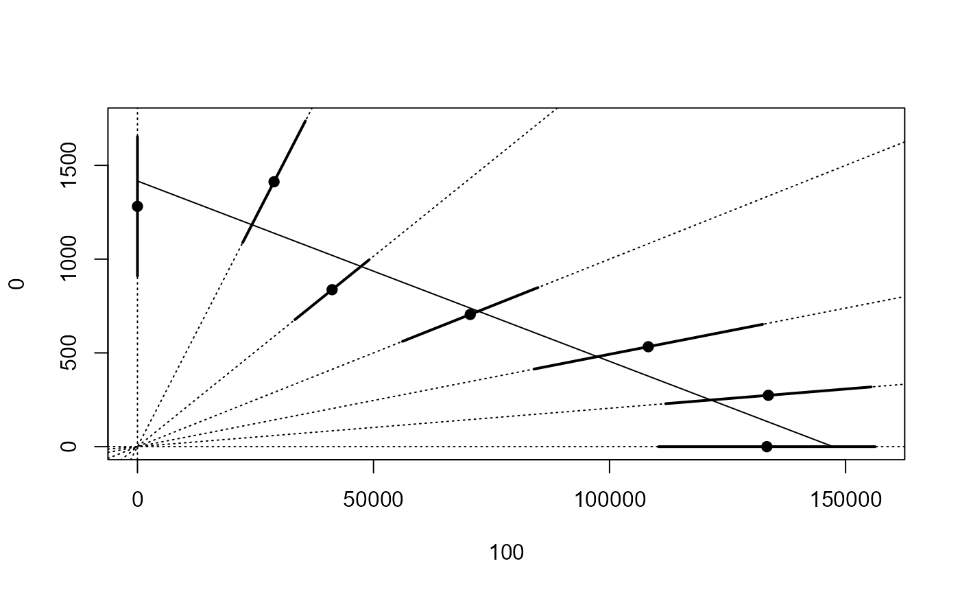
## Plotting isobole structure
isobole(glymet.free, exchange=0.01)
## Fitting the concentration addition model
glymet.ca <- mixture(glymet.free, model = "CA")
#> Warning: Using formula(x) is deprecated when x is a character vector of length > 1.
#> Consider formula(paste(x, collapse = " ")) instead.
#> Control measurements detected for level: 999
## Comparing to model with freely varying e parameter
anova(glymet.ca, glymet.free) # borderline accepted
#>
#> 1st model
#> fct: CA model
#> pmodels: ~~~factor(pct), ~1, ~I(1/(pct/100)) - 1, ~I(1/(1 - pct/100)) - 1
#> 2nd model
#> fct: LL.3()
#> pmodels: ~factor(pct), ~1, ~factor(pct)
#>
#> ANOVA table
#>
#> ModelDf RSS Df F value p value
#> 1st model 103 1.4865
#> 2nd model 98 1.3518 5 1.9532 0.0924
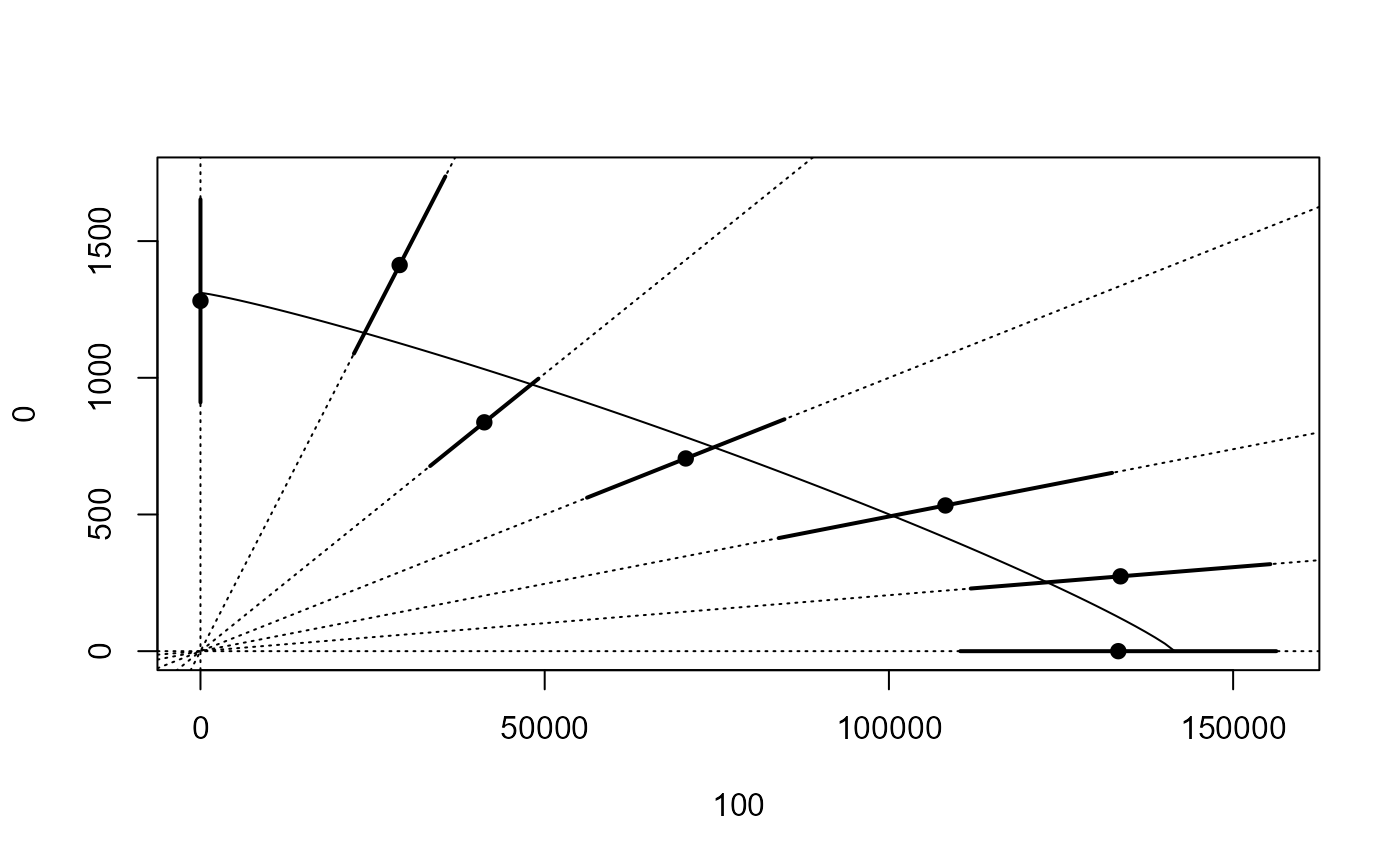
## Plotting isobole based on concentration addition
isobole(glymet.free, glymet.ca, exchange = 0.01) # acceptable fit
 ## Fitting the Hewlett model
glymet.hew <- mixture(glymet.free, model = "Hewlett")
#> Warning: Using formula(x) is deprecated when x is a character vector of length > 1.
#> Consider formula(paste(x, collapse = " ")) instead.
#> Control measurements detected for level: 999
### Comparing to model with freely varying e parameter
anova(glymet.ca, glymet.hew)
#>
#> 1st model
#> fct: CA model
#> pmodels: ~~~factor(pct), ~1, ~I(1/(pct/100)) - 1, ~I(1/(1 - pct/100)) - 1
#> 2nd model
#> fct: Hewlett model
#> pmodels: ~~~factor(pct), ~1, ~I(1/(pct/100)) - 1, ~I(1/(1 - pct/100)) - 1, ~1
#>
#> ANOVA table
#>
#> ModelDf RSS Df F value p value
#> 1st model 103 1.4865
#> 2nd model 102 1.4730 1 0.9360 0.3356
# borderline accepted
# the Hewlett model offers no improvement over concentration addition
## Plotting isobole based on the Hewlett model
isobole(glymet.free, glymet.hew, exchange = 0.01)
## Fitting the Hewlett model
glymet.hew <- mixture(glymet.free, model = "Hewlett")
#> Warning: Using formula(x) is deprecated when x is a character vector of length > 1.
#> Consider formula(paste(x, collapse = " ")) instead.
#> Control measurements detected for level: 999
### Comparing to model with freely varying e parameter
anova(glymet.ca, glymet.hew)
#>
#> 1st model
#> fct: CA model
#> pmodels: ~~~factor(pct), ~1, ~I(1/(pct/100)) - 1, ~I(1/(1 - pct/100)) - 1
#> 2nd model
#> fct: Hewlett model
#> pmodels: ~~~factor(pct), ~1, ~I(1/(pct/100)) - 1, ~I(1/(1 - pct/100)) - 1, ~1
#>
#> ANOVA table
#>
#> ModelDf RSS Df F value p value
#> 1st model 103 1.4865
#> 2nd model 102 1.4730 1 0.9360 0.3356
# borderline accepted
# the Hewlett model offers no improvement over concentration addition
## Plotting isobole based on the Hewlett model
isobole(glymet.free, glymet.hew, exchange = 0.01)
 # no improvement over concentration addition