Plotting fitted dose-response curves

plot displays fitted curves and observations in the same plot window, distinguishing between curves by different plot symbols and line types.

Usage

# S3 method for class 'drc'
plot(
  x,
  ...,
  add = FALSE,
  level = NULL,
  type = c("average", "all", "bars", "none", "obs", "confidence"),
  broken = FALSE,
  bp,
  bcontrol = NULL,
  conName = NULL,
  axes = TRUE,
  gridsize = 100,
  log = "x",
  xtsty,
  xttrim = TRUE,
  xt = NULL,
  xtlab = NULL,
  xlab,
  xlim,
  yt = NULL,
  ytlab = NULL,
  ylab,
  ylim,
  cex,
  cex.axis = 1,
  col = FALSE,
  lty,
  pch,
  legend,
  legendText,
  legendPos,
  cex.legend = 1,
  normal = FALSE,
  normRef = 1,
  confidence.level = 0.95
)

Arguments

x: an object of class 'drc'.
...: additional graphical arguments. For instance, use lwd=2 or lwd=3 to increase the width of plot symbols.
add: logical. If TRUE then add to already existing plot.
level: vector of character strings. To plot only the curves specified by their names.
type: a character string specifying how to plot the data. Options are: "average" (averages and fitted curve(s); default), "none" (only the fitted curve(s)), "obs" (only the data points), "all" (all data points and fitted curve(s)), "bars" (averages and fitted curve(s) with model-based standard errors), and "confidence" (confidence bands for fitted curve(s)).
broken: logical. If TRUE the x axis is broken provided this axis is logarithmic (using functionality in the CRAN package 'plotrix').
bp: numeric value specifying the break point below which the dose is zero. The default is the base-10 value corresponding to the rounded value of the minimum of the log10 values of all positive dose values. Only works for logarithmic dose axes.
bcontrol: a list with components factor, style and width controlling the appearance of the break (when broken is TRUE).
conName: character string. Name on x axis for dose zero. Default is "0".
axes: logical indicating whether both axes should be drawn on the plot.
gridsize: numeric. Number of points in the grid used for plotting the fitted curves.
log: a character string which contains "x" if the x axis is to be logarithmic, "y" if the y axis is to be logarithmic and "xy" or "yx" if both axes are to be logarithmic. The default is "x". The empty string "" yields the original axes.
xtsty: a character string specifying the dose axis style for arrangement of tick marks. By default for a logarithmic axis only base 10 tick marks are shown ("base10"). Otherwise sensible equidistantly located tick marks are shown ("standard").
xttrim: logical specifying if the number of tick marks should be trimmed in case too many tick marks are initially determined.
xt: a numeric vector containing the positions of the tick marks on the x axis.
xtlab: a vector containing the tick marks on the x axis.
xlab: an optional label for the x axis.
xlim: a numeric vector of length two, containing the lower and upper limit for the x axis.
yt: a numeric vector containing the positions of the tick marks on the y axis.
ytlab: a vector containing the tick marks on the y axis.
ylab: an optional label for the y axis.
ylim: a numeric vector of length two, containing the lower and upper limit for the y axis.
cex: numeric or numeric vector specifying the size of plotting symbols and text (see par for details).
cex.axis: numeric value specifying the magnification to be used for axis annotation relative to the current setting of cex.
col: either logical or a vector of colours. If TRUE default colours are used. If FALSE (default) no colours are used.
lty: a numeric vector specifying the line types.
pch: a vector of plotting characters or symbols (see points).
legend: logical. If TRUE a legend is displayed.
legendText: a character string or vector of character strings specifying the legend text.
legendPos: numeric vector of length 2 giving the position of the legend.
cex.legend: numeric specifying the legend text size.
normal: logical. If TRUE the plot of the normalized data and fitted curves are shown (see Weimer et al. (2012) for details).
normRef: numeric specifying the reference for the normalization (default is 1).
confidence.level: confidence level for error bars. Defaults to 0.95.

Value

An invisible data frame with the values used for plotting the fitted curves. The first column contains the dose values, and the following columns (one for each curve) contain the fitted response values.

Details

The use of xlim allows changing the range of the x axis, extrapolating the fitted dose-response curves. Note that changing the range on the x axis may also entail a change of the range on the y axis. Sometimes it may be useful to extend the upper limit on the y axis (using ylim) in order to fit a legend into the plot.

See colors for the available colours. Suitable labels are automatically provided.

The arguments broken and bcontrol rely on the function axis.break with arguments style and brw in the package plotrix.

The model-based standard errors used for the error bars are calculated as the fitted value plus/minus the estimated error times the 1-(alpha/2) quantile in the t distribution with degrees of freedom equal to the residual degrees of freedom for the model (or using a standard normal distribution in case of binomial and Poisson data), where alpha = 1 - confidence.level. The standard errors are obtained using the predict method with the arguments interval = "confidence" and level = confidence.level.

Author

Christian Ritz and Jens C. Streibig. Contributions from Xiaoyan Wang and Greg Warnes.

Examples

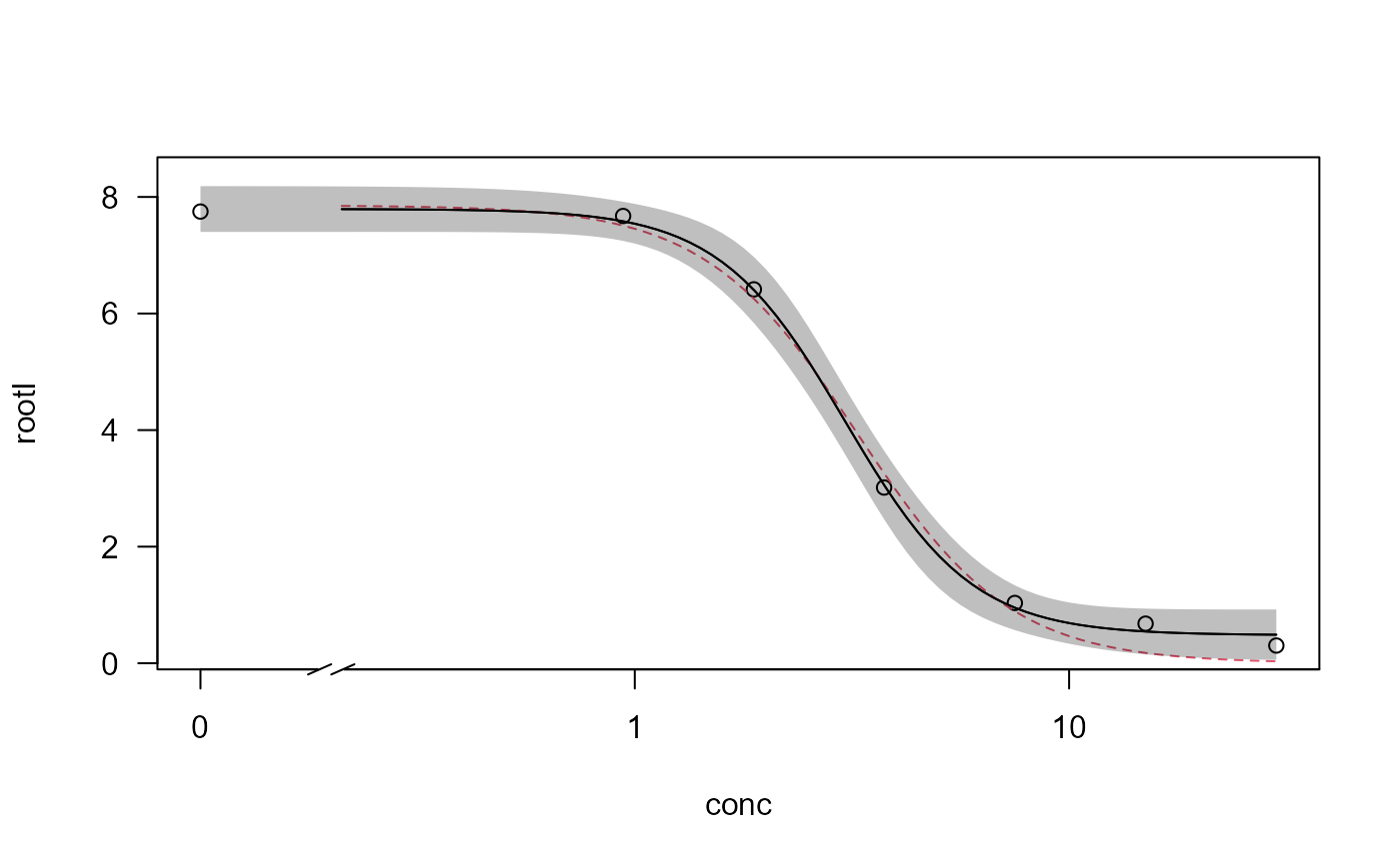
## Fitting models to be plotted below
ryegrass.m1 <- drm(rootl~conc, data = ryegrass, fct = LL.4())
ryegrass.m2 <- drm(rootl~conc, data = ryegrass, fct = LL.3())

## Plotting observations and fitted curve for the first model
plot(ryegrass.m1, broken = TRUE)

## Adding fitted curve for the second model
plot(ryegrass.m2, broken = TRUE, add = TRUE, type = "none", col = 2, lty = 2)

## Add confidence region for the first model
plot(ryegrass.m1, broken = TRUE, type="confidence", add=TRUE)


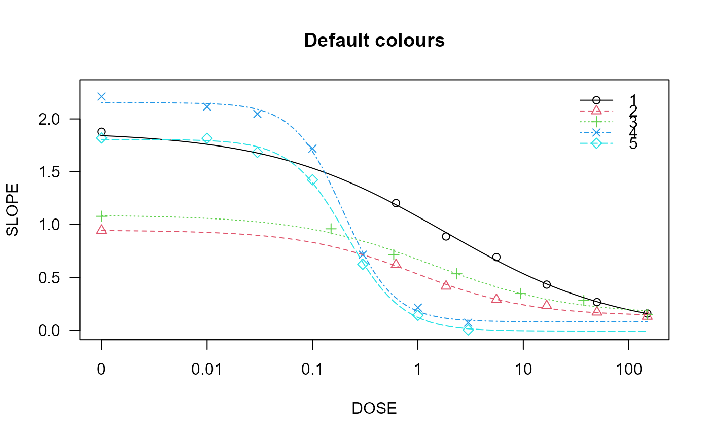
## Fitting model with multiple curves
spinach.m1 <- drm(SLOPE~DOSE, CURVE, data = spinach, fct = LL.4())

## Plot with default colours
plot(spinach.m1, col = TRUE, main = "Default colours")