Red fescue — red.fescue • drc

Data from a dose-response experiment with red fescue (Festuca rubra). Biomass was measured at different dose levels and at two time points (day 0 and day 16).

Usage

data(red.fescue)

Format

A data frame with 26 observations on the following 3 variables.

dose: a numeric vector
day: a numeric vector
biomass: a numeric vector

Examples

library(drc)

## Displaying the data
head(red.fescue)
#>   dose day biomass
#> 1    0   0    45.0
#> 2    0   0    69.0
#> 3    0  16   137.0
#> 4    0  16   102.0
#> 5    0  16   101.4
#> 6   87  16   139.7

## Fitting a four-parameter log-logistic model with separate curves per day
red.fescue.m1 <- drm(biomass ~ dose, day, data = red.fescue, fct = LL.4())
#> Control measurements detected for level: 0
summary(red.fescue.m1)
#> 
#> Model fitted: Log-logistic (ED50 as parameter) (4 parms)
#> 
#> Parameter estimates:
#> 
#>               Estimate Std. Error t-value   p-value    
#> b:(Intercept)   2.2098     1.0445  2.1156   0.04594 *  
#> c:(Intercept)  26.2056    12.0292  2.1785   0.04037 *  
#> d:(Intercept) 109.0601     8.6786 12.5666 1.631e-11 ***
#> e:(Intercept) 456.5766   185.6060  2.4599   0.02222 *  
#> ---
#> Signif. codes:  0 '***' 0.001 '**' 0.01 '*' 0.05 '.' 0.1 ' ' 1
#> 
#> Residual standard error:
#> 
#>  25.21797 (22 degrees of freedom)

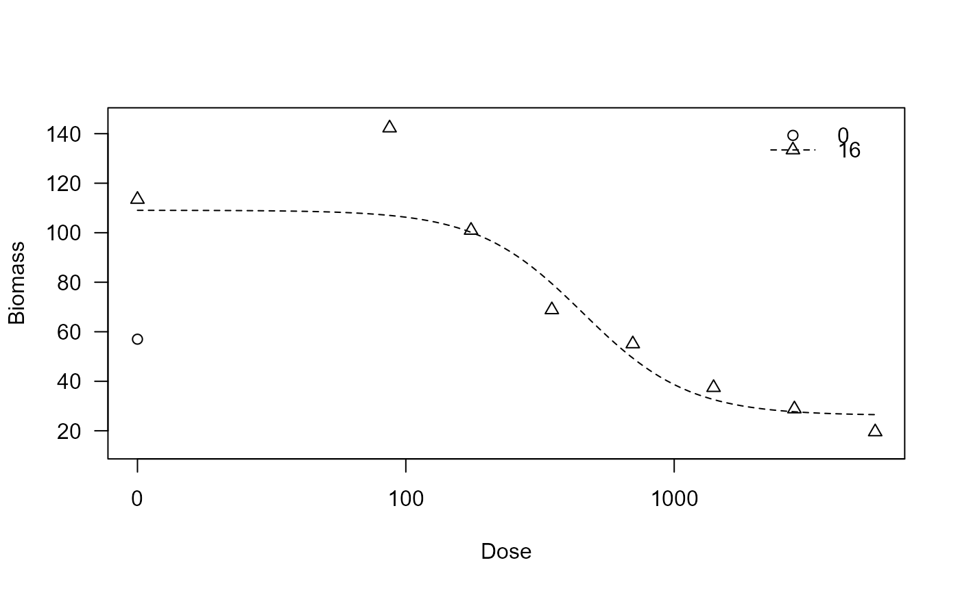
## Plotting the fitted curves
plot(red.fescue.m1, xlab = "Dose", ylab = "Biomass")