Root length measurements

Data stem from an experiment assessing the inhibitory effect of secalonic acids on plant growth.

Usage

data(secalonic)

Format

A data frame with 7 observations on the following 2 variables:

dose

a numeric vector containing dose values (mM)

rootl

a numeric vector containing root lengths (cm)

Details

For each dose the root length is an average three measurements.

Source

Gong, X. and Zeng, R. and Luo, S. and Yong, C. and Zheng, Q. (2004) Two new secalonic acids from Aspergillus Japonicus and their allelopathic effects on higher plants, Proceedings of International Symposium on Allelopathy Research and Application, 27-29 April, Shanshui, Guangdong, China (Editors: R. Zeng and S. Luo), 209–217.

Ritz, C (2009) Towards a unified approach to dose-response modeling in ecotoxicology To appear in Environ Toxicol Chem.

Examples

library(drc)

## Fitting a four-parameter log-logistic model
secalonic.m1 <- drm(rootl ~ dose, data = secalonic, fct = LL.4())
summary(secalonic.m1)
#> 
#> Model fitted: Log-logistic (ED50 as parameter) (4 parms)
#> 
#> Parameter estimates:
#> 
#>                Estimate Std. Error t-value   p-value    
#> b:(Intercept) 2.6542086  0.6962333  3.8122 0.0317398 *  
#> c:(Intercept) 0.0917852  0.3747246  0.2449 0.8223012    
#> d:(Intercept) 5.5297495  0.2010300 27.5071 0.0001055 ***
#> e:(Intercept) 0.0803547  0.0078829 10.1935 0.0020121 ** 
#> ---
#> Signif. codes:  0 '***' 0.001 '**' 0.01 '*' 0.05 '.' 0.1 ' ' 1
#> 
#> Residual standard error:
#> 
#>  0.2957497 (3 degrees of freedom)

## Fitting a three-parameter log-logistic model
##  lower limit fixed at 0
secalonic.m2 <- drm(rootl ~ dose, data = secalonic, fct = LL.3())
summary(secalonic.m1)
#> 
#> Model fitted: Log-logistic (ED50 as parameter) (4 parms)
#> 
#> Parameter estimates:
#> 
#>                Estimate Std. Error t-value   p-value    
#> b:(Intercept) 2.6542086  0.6962333  3.8122 0.0317398 *  
#> c:(Intercept) 0.0917852  0.3747246  0.2449 0.8223012    
#> d:(Intercept) 5.5297495  0.2010300 27.5071 0.0001055 ***
#> e:(Intercept) 0.0803547  0.0078829 10.1935 0.0020121 ** 
#> ---
#> Signif. codes:  0 '***' 0.001 '**' 0.01 '*' 0.05 '.' 0.1 ' ' 1
#> 
#> Residual standard error:
#> 
#>  0.2957497 (3 degrees of freedom)

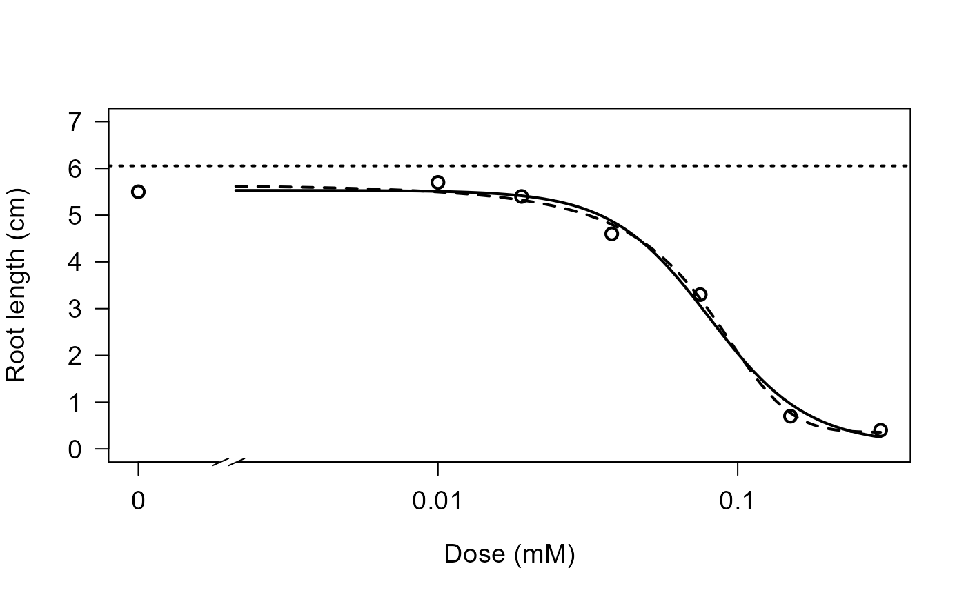
## Comparing logistic and log-logistic models
## (Figure 1 in Ritz (2009))
secalonic.LL4 <- drm(rootl ~ dose, data = secalonic, fct = LL.4())
secalonic.L4 <- drm(rootl ~ dose, data = secalonic, fct = L.4())

plot(secalonic.LL4, broken=TRUE, ylim=c(0,7), xlab="Dose (mM)", ylab="Root length (cm)", 
cex=1.2, cex.axis=1.2, cex.lab=1.2, lwd=2)

plot(secalonic.L4, broken=TRUE, ylim=c(0,7), add=TRUE, type="none", lty=2, lwd=2)

abline(h=coef(secalonic.L4)[3], lty=3, lwd=2)